Creating legends when aesthetics are constants in ggplot2
In general, if you want to map an aesthetic to a variable and get a legend in ggplot2 you do it inside aes(). If you want to set an aesthetic to a constant value, like making all your points purple, you do it outside aes().
However, there are situations where you might want to set an aesthetic for a layer to a constant but you also want a legend for that aesthetic. One common alternative is to put your dataset into a long format to take advantage of the strengths of ggplot2, but that isn’t a straightforward option for every situation. I’ll show another approach here.
Table of Contents
- The setup
- Making a plot with aesthetics as constants
- Why won’t scale_color_manual() make a legend?
- Adding a legend by moving aesthetics into aes()
- Using scale_color_identity() to recognize color strings
- Descriptive strings and scale_color_manual()
- Other examples on Stack Overflow
- Just the code, please
The setup
A few situations where we might want legends without mapping an aesthetic to a variable are:
1. Adding a statistic like the mean as a line or symbol and wanting a legend to define it
2. Adding separate layers for subsets of data or based on different datasets*
3. Adding lines based on different fitted models
*This second situation is where reformatting your dataset is often most useful
Today I’ll focus on adding lines from different models. I’m going to be using the ubiquitous mtcars dataset for the work. 😆
Making a plot with aesthetics as constants
I’ll start by loading the ggplot2 package.
library(ggplot2) # v. 3.2.0I’m going to make a plot of the relationship between mpg and hp, adding three fitted lines from three different linear regression models. I will use a linear, a quadratic, and a cubic model. I use geom_smooth() to make the fitted regression lines, and so add a separate geom_smooth() layer for each model.
I’m going to focus on the color aesthetic here, but this is relevant for other aesthetics, as well.
You can see I set a different color per fitted line. Since I’m setting these colors as constants this is done outside aes().
ggplot(mtcars, aes(mpg, hp) ) +
     geom_point() +
     geom_smooth(method = "lm", se = FALSE, color = "black") +
     geom_smooth(method = "lm", formula = y ~ poly(x, 2), se = FALSE, color = "red") +
     geom_smooth(method = "lm", formula = y ~ poly(x, 3), se = FALSE, color = "blue")
It would be nice to know which line came from which model, and adding a legend is one way to do that. So how can we do this?
Why won’t scale_color_manual() make a legend?
I think for many people it feels intuitive to add the appropriate scale_*() function to the plotting code in hopes of getting a legend. Along those lines I’ll add scale_color_manual() to my plot.
ggplot(mtcars, aes(mpg, hp) ) +
     geom_point() +
     geom_smooth(method = "lm", se = FALSE, color = "black") +
     geom_smooth(method = "lm", formula = y ~ poly(x, 2), se = FALSE, color = "red") +
     geom_smooth(method = "lm", formula = y ~ poly(x, 3), se = FALSE, color = "blue") +
     scale_color_manual(values = c("black", "red", "blue") )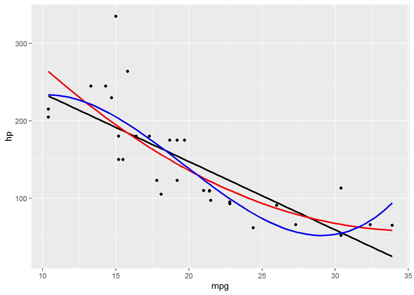
But nothing changes. Unfortunately, no matter how hard I throw scale_color_manual() at the plot, I won’t get a legend in this way.
Why doesn’t this work?
From the description in the scale_manual documentation, the manual scale functions allow you to specify your own set of mappings from levels in the data to aesthetic values. You can change already created mappings but not construct them. In ggplot2, mappings are constructed by aes(). Aesthetics therefore must be inside aes() to get a legend.
Adding a legend by moving aesthetics into aes()
I’ll move color inside of aes() within each geom_smooth() layer to construct color mappings. This adds a legend to the plot.
ggplot(mtcars, aes(mpg, hp) ) +
     geom_point() +
     geom_smooth(method = "lm", se = FALSE, aes(color = "black") ) +
     geom_smooth(method = "lm", formula = y ~ poly(x, 2), se = FALSE, aes(color = "red") ) +
     geom_smooth(method = "lm", formula = y ~ poly(x, 3), se = FALSE, aes(color = "blue") )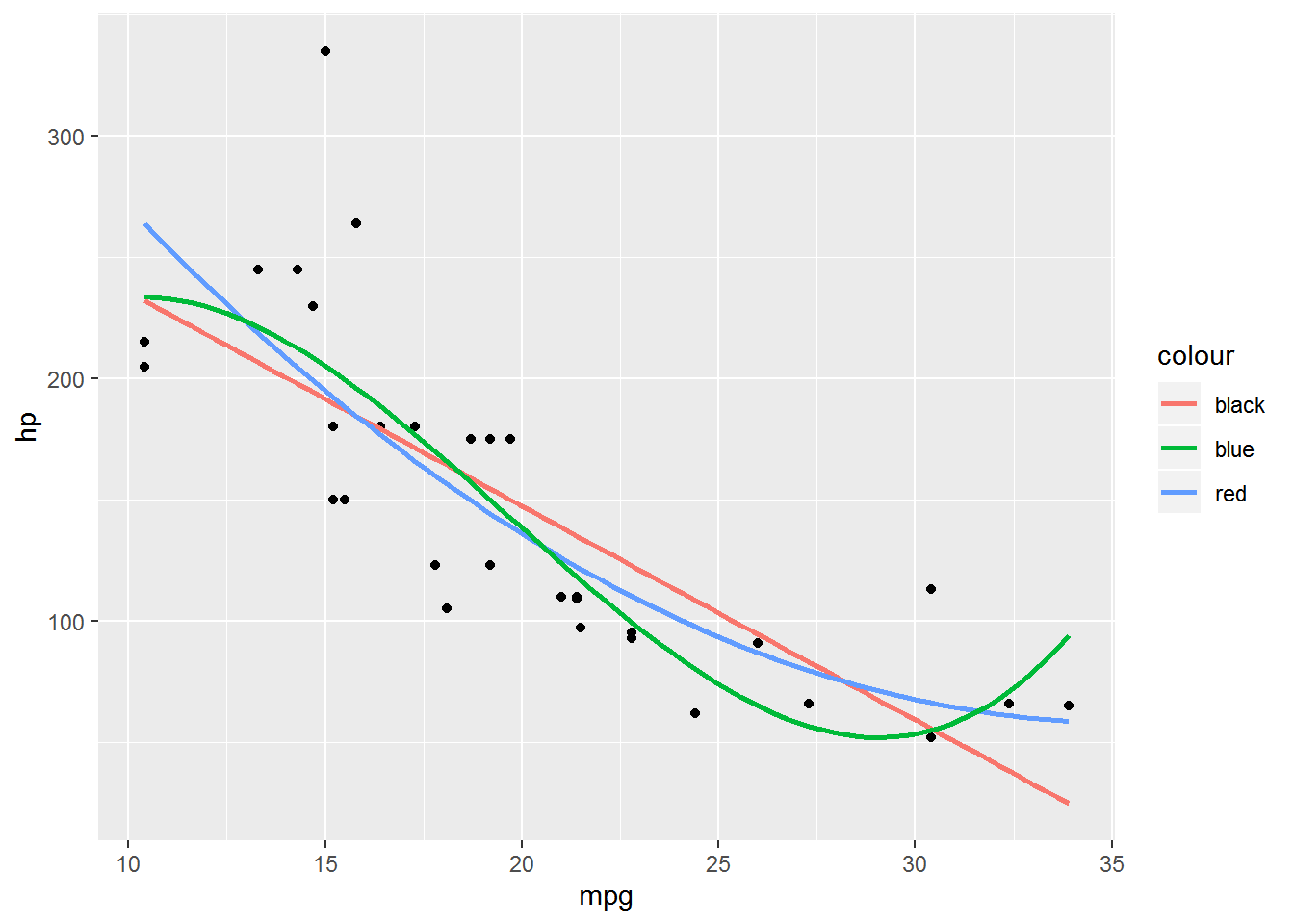
My plot now has a legend 👍, but the colors have changed 👎. The values are no longer recognized as colors since aes() treats these as string constants. To get the desired colors we’ll need to turn to one of the scale_color_*() functions.
Using scale_color_identity() to recognize color strings
One way to force ggplot to recognize the color names when they are inside aes() is to use scale_color_identity(). To get a legend with an identity scale you must use guide = "legend". (The default is guide = "none" for identity scales.)
ggplot(mtcars, aes(mpg, hp) ) +
     geom_point() +
     geom_smooth(method = "lm", se = FALSE, aes(color = "black") ) +
     geom_smooth(method = "lm", formula = y ~ poly(x, 2), se = FALSE, aes(color = "red") ) +
     geom_smooth(method = "lm", formula = y ~ poly(x, 3), se = FALSE, aes(color = "blue") ) +
     scale_color_identity(guide = "legend")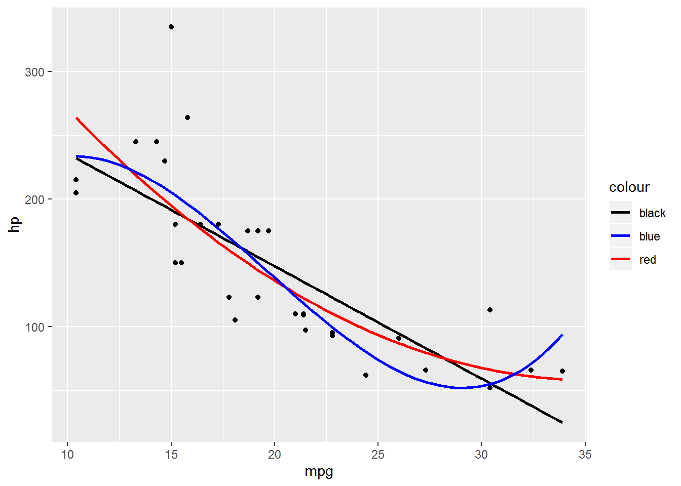
The colors are now correct but the legend still leaves a lot to be desired. The name of the legend isn’t useful, the order is alphabetical instead of by model complexity, and the labels are the color names instead of descriptive names that describe each model.
The legend name can be changed via name, the order can be changes via breaks and the labels can be changed via labels in scale_color_identity(). The order of the labels must be the same as the order of the breaks.
This all means the scale_color_identity() code gets quite a bit more complicated. I’ve found this to be pretty standard when mapping aesthetics to constants.
ggplot(mtcars, aes(mpg, hp) ) +
     geom_point() +
     geom_smooth(method = "lm", se = FALSE, aes(color = "black") ) +
     geom_smooth(method = "lm", formula = y ~ poly(x, 2), se = FALSE, aes(color = "red") ) +
     geom_smooth(method = "lm", formula = y ~ poly(x, 3), se = FALSE, aes(color = "blue") ) +
     scale_color_identity(name = "Model fit",
                          breaks = c("black", "red", "blue"),
                          labels = c("Linear", "Quadratic", "Cubic"),
                          guide = "legend")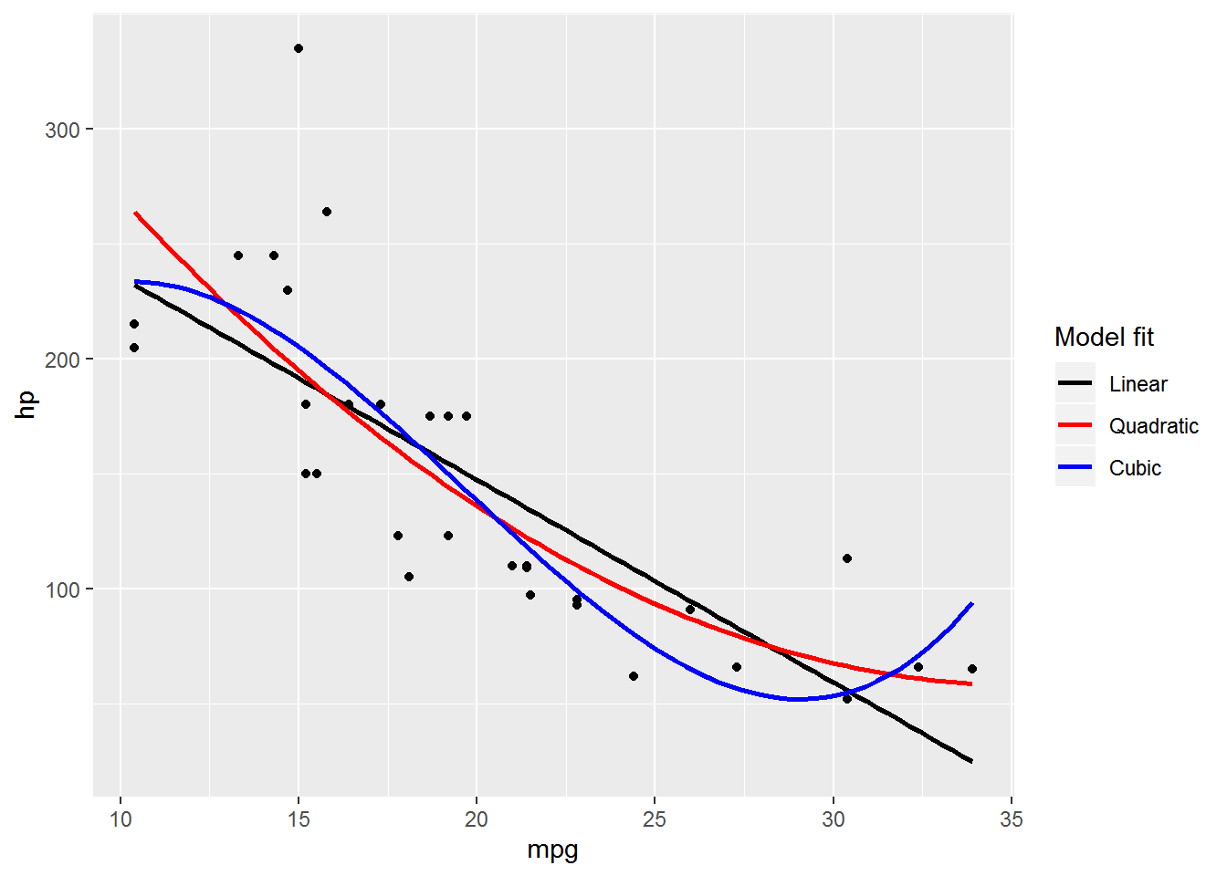
Descriptive strings and scale_color_manual()
An alternative (but not necessarily simpler 😄) approach is to use informative string names instead of the color names within aes(). Then we can use scale_color_manual() to get the legend cleaned up.
Here is the plot using descriptive names that describe each model instead of the color names.
ggplot(mtcars, aes(mpg, hp) ) +
     geom_point() +
     geom_smooth(method = "lm", se = FALSE, aes(color = "Linear") ) +
     geom_smooth(method = "lm", formula = y ~ poly(x, 2), se = FALSE, aes(color = "Quadratic") ) +
     geom_smooth(method = "lm", formula = y ~ poly(x, 3), se = FALSE, aes(color = "Cubic") )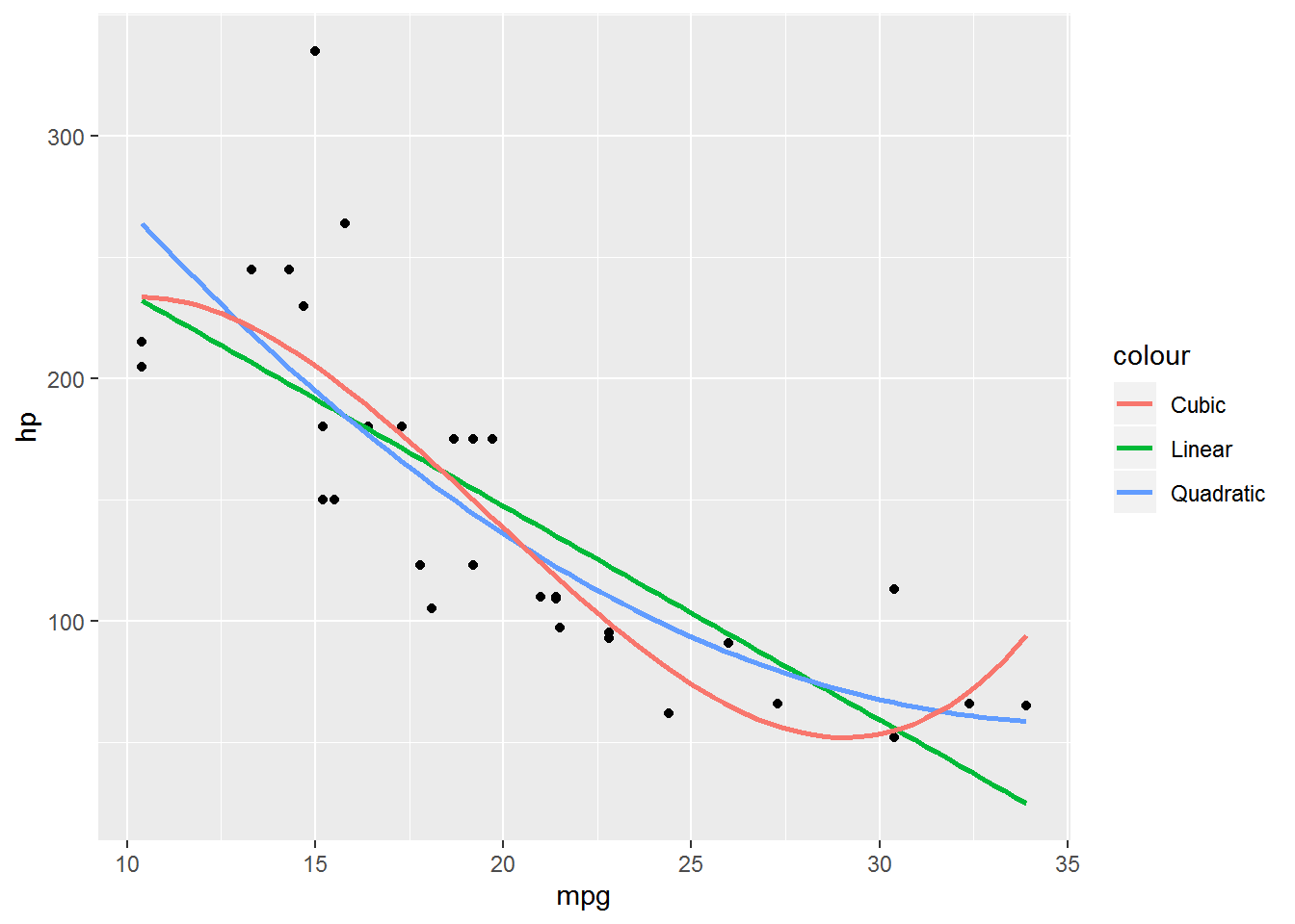
This has nicer labels, but the legend has other problems, similar to those above. The legend name isn’t informative, the order is again alphabetical instead of by model complexity, and the colors still need to be changed if we really want black, red, and blue lines. This can all be addressed in scale_color_manual().
For the first two issues I will again use name and breaks to get things named and in the desired order.
Colors are set via passing a vector of color names to the values argument in scale_color_manual(). Note the values argument is a required aesthetic in scale_color_manual(); if you don’t want to change the colors in the plot use scale_color_discrete().
The vector of colors needs to either be in the same order as the breaks or given as a named vector. The latter is “safest” since it is invariant to changing the order of the legend, and so I’ll use a named vector in my example code.
ggplot(mtcars, aes(mpg, hp) ) +
     geom_point() +
     geom_smooth(method = "lm", se = FALSE, aes(color = "Linear") ) +
     geom_smooth(method = "lm", formula = y ~ poly(x, 2), se = FALSE, aes(color = "Quadratic") ) +
     geom_smooth(method = "lm", formula = y ~ poly(x, 3), se = FALSE, aes(color = "Cubic") ) +
     scale_color_manual(name = "Model fit",
                        breaks = c("Linear", "Quadratic", "Cubic"),
                        values = c("Cubic" = "blue", "Quadratic" = "red", "Linear" = "black") )
Other examples on Stack Overflow
You can see what I would consider some of the canonical questions and answers on this topic from Stack Overflow here and here. (I’m sure there are others, but these are two that I’ve been linking to as duplicates recently. 😺)
Just the code, please
Here’s the code without all the discussion. Copy and paste the code below or you can download an R script of uncommented code from here.
library(ggplot2) # v. 3.2.0

ggplot(mtcars, aes(mpg, hp) ) +
     geom_point() +
     geom_smooth(method = "lm", se = FALSE, color = "black") +
     geom_smooth(method = "lm", formula = y ~ poly(x, 2), se = FALSE, color = "red") +
     geom_smooth(method = "lm", formula = y ~ poly(x, 3), se = FALSE, color = "blue")

ggplot(mtcars, aes(mpg, hp) ) +
     geom_point() +
     geom_smooth(method = "lm", se = FALSE, color = "black") +
     geom_smooth(method = "lm", formula = y ~ poly(x, 2), se = FALSE, color = "red") +
     geom_smooth(method = "lm", formula = y ~ poly(x, 3), se = FALSE, color = "blue") +
     scale_color_manual(values = c("black", "red", "blue") )

ggplot(mtcars, aes(mpg, hp) ) +
     geom_point() +
     geom_smooth(method = "lm", se = FALSE, aes(color = "black") ) +
     geom_smooth(method = "lm", formula = y ~ poly(x, 2), se = FALSE, aes(color = "red") ) +
     geom_smooth(method = "lm", formula = y ~ poly(x, 3), se = FALSE, aes(color = "blue") )

ggplot(mtcars, aes(mpg, hp) ) +
     geom_point() +
     geom_smooth(method = "lm", se = FALSE, aes(color = "black") ) +
     geom_smooth(method = "lm", formula = y ~ poly(x, 2), se = FALSE, aes(color = "red") ) +
     geom_smooth(method = "lm", formula = y ~ poly(x, 3), se = FALSE, aes(color = "blue") ) +
     scale_color_identity(guide = "legend")

ggplot(mtcars, aes(mpg, hp) ) +
     geom_point() +
     geom_smooth(method = "lm", se = FALSE, aes(color = "black") ) +
     geom_smooth(method = "lm", formula = y ~ poly(x, 2), se = FALSE, aes(color = "red") ) +
     geom_smooth(method = "lm", formula = y ~ poly(x, 3), se = FALSE, aes(color = "blue") ) +
     scale_color_identity(name = "Model fit",
                          breaks = c("black", "red", "blue"),
                          labels = c("Linear", "Quadratic", "Cubic"),
                          guide = "legend")

ggplot(mtcars, aes(mpg, hp) ) +
     geom_point() +
     geom_smooth(method = "lm", se = FALSE, aes(color = "Linear") ) +
     geom_smooth(method = "lm", formula = y ~ poly(x, 2), se = FALSE, aes(color = "Quadratic") ) +
     geom_smooth(method = "lm", formula = y ~ poly(x, 3), se = FALSE, aes(color = "Cubic") )

ggplot(mtcars, aes(mpg, hp) ) +
     geom_point() +
     geom_smooth(method = "lm", se = FALSE, aes(color = "Linear") ) +
     geom_smooth(method = "lm", formula = y ~ poly(x, 2), se = FALSE, aes(color = "Quadratic") ) +
     geom_smooth(method = "lm", formula = y ~ poly(x, 3), se = FALSE, aes(color = "Cubic") ) +
     scale_color_manual(name = "Model fit",
                        breaks = c("Linear", "Quadratic", "Cubic"),
                        values = c("Cubic" = "blue", "Quadratic" = "red", "Linear" = "black") )