Using DHARMa for residual checks of unsupported models
One of the difficult things about working with generalized linear models (GLM) and generalized linear mixed models (GLMM) is figuring out how to interpret residual plots. We don’t really expect residual plots from a GLMM to look like one from a linear model, sure, but how do we tell when something looks “bad”?
This is the situation I was in several years ago, working on an analysis involving counts from a fairly complicated study design. I was using a negative binomial generalized linear mixed models, and the residual vs fitted values plot looked, well, “funny”. But I wasn’t sure if something was wrong or if this was just how the residuals from a complicated model like this looked sometimes. At this point I dipped my toe into using simulations for model checking for the first time.
Table of Contents
Why use simulations for model checking?
Here is an example of a plot I wasn’t feeling too good about but also wasn’t certain if what I was seeing indicated a lack of fit.
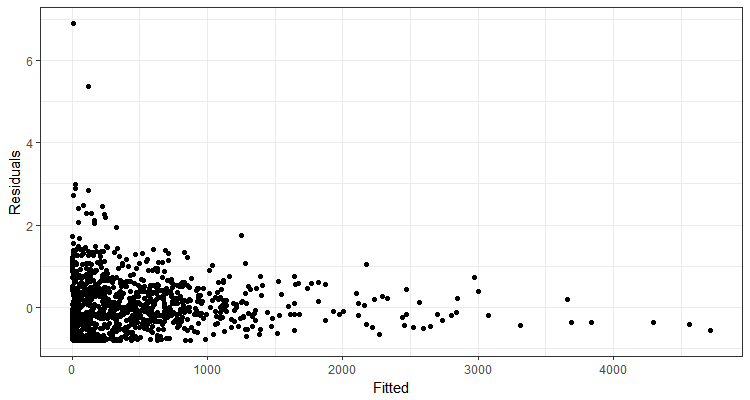
To try to figure out if what I was seeing was a problem, I fit models to response data simulated from my model. The beauty of such simulations is that I know that the model definitely does fit the simulated response data; the model is what created the data! I compared residuals plots from simulated data models to my real plot to help decide if what I was seeing was unusual. I looked at a fair number of simulated residual plots and decided that, yes, something was wrong with my model. I ended up moving on to a different model that worked better.
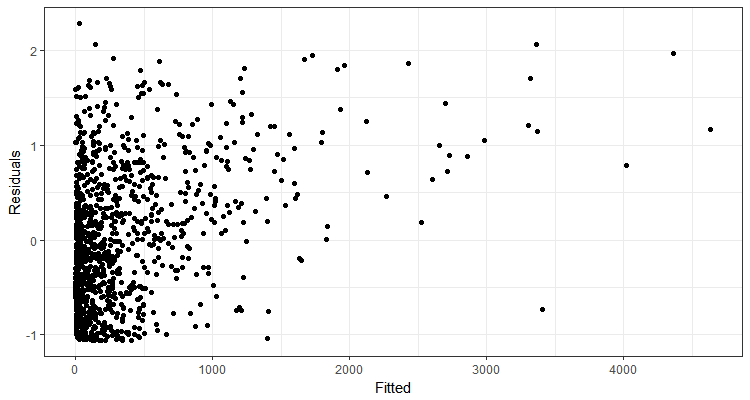
Here is an example of one of the simulated residual plots. There was definitely variation in plots from models fit to the simulated data, but this is a good example of what they generally looked like.
The DHARMa package
I found my “brute force” simulation approach useful, but I spent a lot of time visually comparing the simulated plots to my real plot. I didn’t have a metric to help me decide if my actual residual plot seemed unusual compared to residual plots from my “true” models. This left me unable to recommend this as a general approach to folks I consult with.
Since then, the author of the DHARMa package has come up with a clever way to use a simulation-based approach for residuals checks of GLMM’s. If you are interested in trying the package out, it has a very nice vignette to get you started.
These days I’m been happily recommending the DHARMa packages to students I work with for residual checks of GLMM’s. However, students aren’t always working with models that DHARMa currently supports. Luckily, DHARMa can simulate residuals for any model as long as the user can provide simulated values to the createDHARMa() function. Below I show how to do this for a couple of different situations.
How to use createDHARMa()
In order to use createDHARMa(), the user needs to provide three pieces of information.
- Simulated response vectors
- Observed data
- The predicted response from the model
I thinking making the simulated response vectors is the biggest bottleneck for folks I’ve worked with, and that is what I’m focusing on today.
Simulations for models that have a simulate() function
When a function has a simulate() function, getting the simulations needed to use createDHARMa() can be comparatively straightforward.
Example using glmmTMB()
The glmmTMB() function from package glmmTMB is one of those models that DHARMa doesn’t currently support. (2018-04-05 update: the development version of DHARMA now supports glmmTMB objects for glmmTMB 0.2.1. I believe the example below is still useful for showing how to work with DHARMa-unsupported model types that have a simulate() function.)
There is a simulate() function for glmmTMB objects.
library(DHARMa) # version 0.1.5
library(glmmTMB) # version 0.1.1
I’m going to use one of the models from the glmmTMB documentation to demonstrate how to make the simulations and then use them in createDHARMa().
Below I fit zero-inflated negative binomial model with glmmTMB().
fit_nbz = glmmTMB(count ~ spp + mined + (1|site),
                  zi = ~spp + mined,
                  family = nbinom2, data = Salamanders)
If you try to calculate the scaled residuals via DHARMa functions for an unsupported model, you will get a warning and then an error. DHARMa attempts to make predictions from the model to simulate with, but it will then fail.
This is an indication that you’d to use createDHARMa() to make the residuals instead.
I can simulate from my model via the simulate() function (see the documentation for ?simulate.glmmTMB for details). I usually do at least 1000 simulations if it isn’t too time-consuming. I’ll do only 10 here as an example.
sim_nbz = simulate(fit_nbz, nsim = 10)The result is a list of simulated response vectors.
str(sim_nbz)# 'data.frame': 644 obs. of 10 variables:
# $ sim_1 : num 1 1 0 0 2 0 1 0 14 1 ...
# $ sim_2 : num 0 0 0 2 0 1 2 0 6 5 ...
# $ sim_3 : num 0 0 0 1 3 1 2 0 0 0 ...
# $ sim_4 : num 0 0 0 0 1 3 6 0 3 1 ...
# $ sim_5 : num 1 0 5 0 1 3 2 5 2 2 ...
# $ sim_6 : num 0 0 0 2 1 2 0 1 9 0 ...
# $ sim_7 : num 0 0 0 0 3 4 6 0 0 0 ...
# $ sim_8 : num 0 0 0 1 0 1 0 3 2 3 ...
# $ sim_9 : num 0 0 0 0 1 0 4 0 3 9 ...
# $ sim_10: num 0 0 0 0 2 1 1 2 3 12 ...
# - attr(*, "seed")= int 10403 1 -537199090 444372601 -1868766709 1060936506 -1912847812 -237895297 1019579093 -2071819540 ...I need these in a matrix, not a list, where each column contains a simulated response vector and each row is an observation. I’ll collapse the list into a matrix by using cbind() in do.call.
sim_nbz = do.call(cbind, sim_nbz)
head(sim_nbz)
# sim_1 sim_2 sim_3 sim_4 sim_5 sim_6 sim_7 sim_8 sim_9 sim_10
# [1,] 1 0 0 0 1 0 0 0 0 0
# [2,] 1 0 0 0 0 0 0 0 0 0
# [3,] 0 0 0 0 5 0 0 0 0 0
# [4,] 0 2 1 0 0 2 0 1 0 0
# [5,] 2 0 3 1 1 1 3 0 1 2
# [6,] 0 1 1 3 3 2 4 1 0 1Now I can pass these to createDHARMa() along with observed values and model predictions. I set integerResponse to TRUE, as well, as I’m working with counts.
sim_res_nbz = createDHARMa(simulatedResponse = sim_nbz,
                           observedResponse = Salamanders$count,
                           fittedPredictedResponse = predict(fit_nbz),
                           integerResponse = TRUE)
This function creates the scaled residuals that can be used to make residual plots via DHARMa’s plotSimulatedResiduals(). (In current versions of DHARMa just use plot() instead of plotSimulatedResiduals().)
Remember I’ve only done 10 simulations here, so this particular set of plots don’t look very nice.
plotSimulatedResiduals(sim_res_nbz)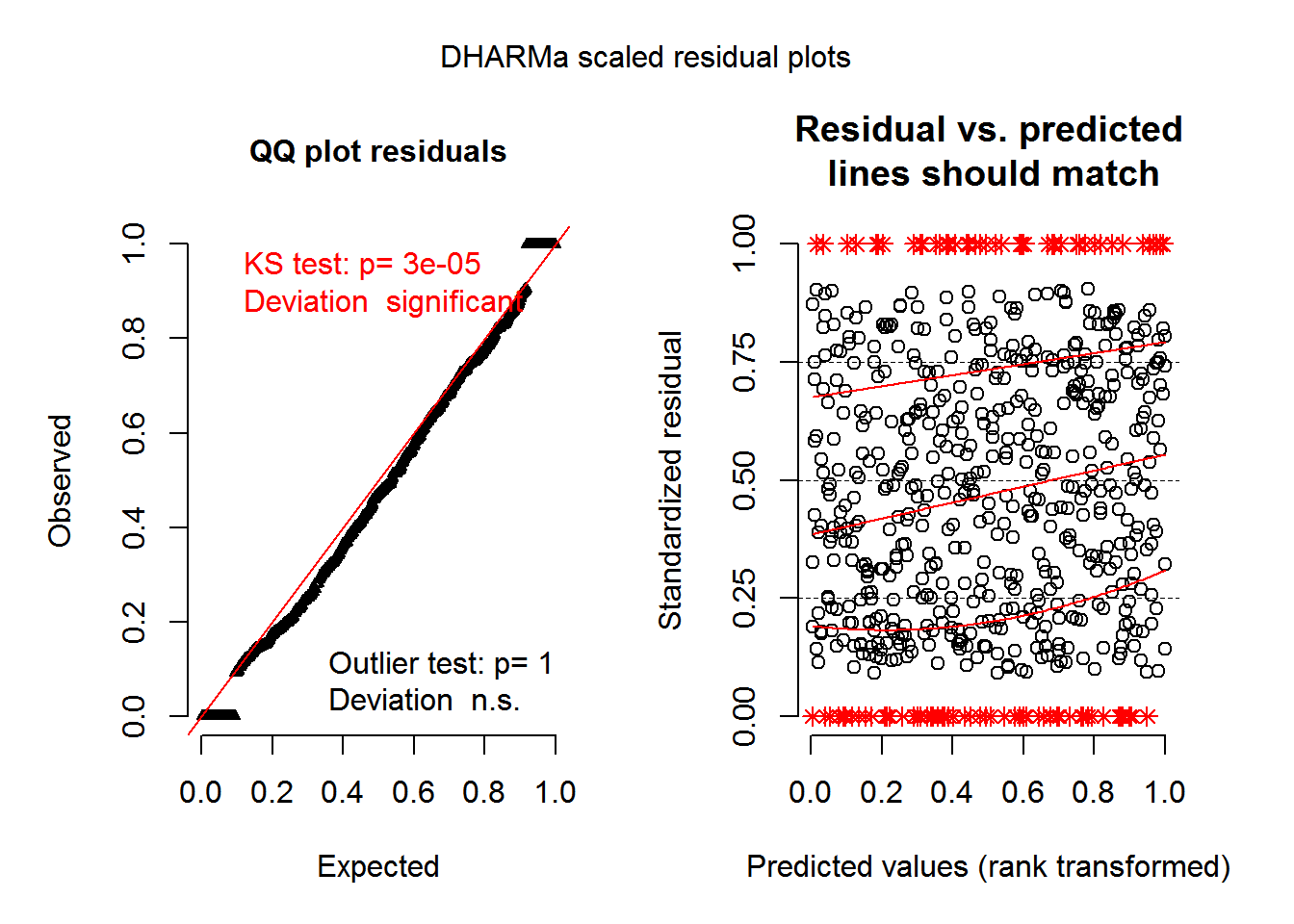
Simulations for models without a simulate() function
The simulate() function did most of the heavy lifting for me in the glmmTMB example. Not all models have a simulate() function, though. This doesn’t mean I can’t use DHARMa, but it does mean I have to put more effort in up front.
I will do the following simulations“by hand” in R, more-or-less following the method shown in this answer on CrossValidated.
Example using zeroinfl()
The zeroinfl() function from package pscl is an example of a model that doesn’t have a simulate() function and is unsupported by DHARMa. I will use this in my next example.
I will also load package VGAM, which has a function for making random draws from a zero-inflated negative binomial distribution.
library(pscl) # version 1.5.2
library(VGAM) # version 1.0-4
I will use a zeroinfl() documentation example in this section. The zero-inflated negative binomial model is below.
fit_zinb = zeroinfl(art ~ . | 1,
                    data = bioChemists,
                    dist = "negbin")
In order to make my own simulations, I’ll need both the model-predicted count and the model-predicted probability of a 0 for each observation in the dataset. I’ll also need an estimate of the negative binomial dispersion parameter, \(\theta\).
The predict() function for zeroinfl models lets the user define the kind of prediction desired. I use predict() twice, once to extra the predicted counts and once to extract the predicted probability of 0.
# Predicted probabilities
p = predict(fit_zinb, type = "zero")
# Predicted counts
mus = predict(fit_zinb, type = "count")
I can pull \(\theta\) directly out of the model output.
fit_zinb$theta# [1] 2.264391Now that I have these, I can make random draws from a zero-inflated negative distribution using rzinegbin from package VGAM.
It took me awhile to figure out which arguments I needed to use in rzinegbin. I need to provide the predicted counts to the "munb" argument and the predicted probabilities to the "pstr0" argument. The "size" argument is the estimate of the dispersion parameter. And the "n" arguments indicates the number of simulated values needed, in this case the same number as the rows in the original dataset.
sim1 = rzinegbin(n = nrow(bioChemists),
                 size = fit_zinb$theta,
                 pstr0 = p,
                 munb = mus)
I use replicate() to draw more than one simulated vector. The first argument of replicate(), "n", indicates the number of times to evaluate the given expression. Here I make 10 simulated response vectors.
sim_zinb = replicate(10, rzinegbin(n = nrow(bioChemists),
                                   size = fit_zinb$theta,
                                   pstr0 = p,
                                   munb = mus) )
The output of replicate() in this case is a matrix, with one simulated response vector in every column and an observation in every row. This is ready for use in createDHARMa().
head(sim_zinb)# [,1] [,2] [,3] [,4] [,5] [,6] [,7] [,8] [,9] [,10]
# [1,] 3 1 1 1 3 3 0 4 1 1
# [2,] 0 0 2 0 0 1 1 2 1 0
# [3,] 0 0 4 0 0 0 1 0 3 0
# [4,] 1 3 0 6 0 0 4 5 1 0
# [5,] 7 4 4 5 1 3 3 5 7 0
# [6,] 0 0 5 0 0 0 0 1 4 1Making the simulations was the hard part. Now that I have them, createDHARMa() works exactly the same way as in the glmmTMB example.
sim_res_zinb = createDHARMa(simulatedResponse = sim_zinb,
                            observedResponse = bioChemists$art,
                            fittedPredictedResponse = predict(fit_zinb, type = "response"),
                            integerResponse = TRUE)
plotSimulatedResiduals(sim_res_zinb)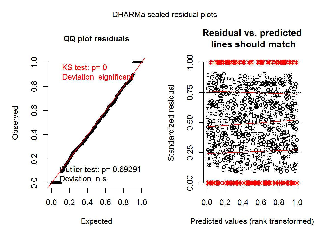
Just the code, please
Here’s the code without all the discussion. Copy and paste the code below or you can download an R script of uncommented code from here.
library(DHARMa) # version 0.1.5
library(glmmTMB) # version 0.1.1

fit_nbz = glmmTMB(count ~ spp + mined + (1|site),
                  zi = ~spp + mined,
                  family = nbinom2, data = Salamanders)

sim_nbz = simulate(fit_nbz, nsim = 10)
str(sim_nbz)

sim_nbz = do.call(cbind, sim_nbz)
head(sim_nbz)

sim_res_nbz = createDHARMa(simulatedResponse = sim_nbz,
                           observedResponse = Salamanders$count,
                           fittedPredictedResponse = predict(fit_nbz),
                           integerResponse = TRUE)
plotSimulatedResiduals(sim_res_nbz)

library(pscl) # version 1.5.2
library(VGAM) # version 1.0-4

fit_zinb = zeroinfl(art ~ . | 1,
                    data = bioChemists,
                    dist = "negbin")

# Predicted probabilities
p = predict(fit_zinb, type = "zero")
# Predicted counts
mus = predict(fit_zinb, type = "count")
fit_zinb$theta

sim1 = rzinegbin(n = nrow(bioChemists),
                 size = fit_zinb$theta,
                 pstr0 = p,
                 munb = mus)

sim_zinb = replicate(10, rzinegbin(n = nrow(bioChemists),
                                   size = fit_zinb$theta,
                                   pstr0 = p,
                                   munb = mus) )
head(sim_zinb)

sim_res_zinb = createDHARMa(simulatedResponse = sim_zinb,
                            observedResponse = bioChemists$art,
                            fittedPredictedResponse = predict(fit_zinb, type = "response"),
                            integerResponse = TRUE)
plotSimulatedResiduals(sim_res_zinb)