The gas mileage data

We record gas mileage for all our vehicles on Google Sheets, so I can read the data in directly from there.

library(googlesheets) # v 0.2.2
library(skimr) # v. 1.0.1
library(dplyr) # v. 0.7.4

The workbook has a sheet for every year of ownership (into the future! 😆) plus service records.

gs_title("Fiesta mpg")

## Sheet successfully identified: "Fiesta mpg"

##                   Spreadsheet title: Fiesta mpg
##                  Spreadsheet author: skylarkguy
##   Date of googlesheets registration: 2018-08-17 01:01:45 GMT
##     Date of last spreadsheet update: 2018-08-16 01:56:05 GMT
##                          visibility: private
##                         permissions: rw
##                             version: new
## 
## Contains 6 worksheets:
## (Title): (Nominal worksheet extent as rows x columns)
## 2016: 1000 x 26
## Service records: 1000 x 26
## 2017: 1000 x 26
## 2018: 1000 x 26
## 2019: 1000 x 26
## 2020: 1000 x 26
## 
## Key: 1xzNrd6c3sWYIxPciREz3nmY8hcol4KJ5qekNqvXyLso
## Browser URL: https://docs.google.com/spreadsheets/d/1xzNrd6c3sWYIxPciREz3nmY8hcol4KJ5qekNqvXyLso/

fiesta2017 = gs_title("Fiesta mpg") %>%
     gs_read("2017")

## Sheet successfully identified: "Fiesta mpg"

## Accessing worksheet titled '2017'.

## Parsed with column specification:
## cols(
##   date = col_character(),
##   gallons = col_double(),
##   cost = col_double(),
##   mileage = col_double(),
##   mpggage = col_double(),
##   mpgcalc = col_double()
## )

We calculate gas mileage (mpgcalc) based on recorded gallons and mileage driven every time we get gas. We also record what the car estimated the gas mileage would be (mpggage).

head(fiesta2017)

## # A tibble: 6 x 6
##   date      gallons  cost mileage mpggage mpgcalc
##   <chr>       <dbl> <dbl>   <dbl>   <dbl>   <dbl>
## 1 1/2/2017     9.78  24.0    359.    38.3    36.8
## 2 1/10/2017    8.87  22.2    330.    38.2    37.2
## 3 1/17/2017   10.4   25.9     NA     39.2     0  
## 4 1/20/2017    7.15  17.7    297.    40.6    41.6
## 5 1/24/2017    7.96  19.7    311.    40.4    39.1
## 6 1/30/2017    9.60  23.6    386.    41.1    40.2

Here’s my first chance to use functions from package skimr to get a quick summary of the variables in the dataset. (I’ve removed the spark histograms since I haven’t gotten them to play nicely in HTML.)

skim(fiesta2017)

## Skim summary statistics
##  n obs: 64 
##  n variables: 6 
## 
## -- Variable type:character ---------------------------------------------------
##  variable missing complete  n min max empty n_unique
##      date       0       64 64   8  10     0       62
## 
## -- Variable type:numeric -----------------------------------------------------
##  variable missing complete  n   mean    sd     p0    p25    p50    p75
##      cost       0       64 64  23.75  3.68  12.23  22.65  24.05  26.39
##   gallons       0       64 64   8.83  1.33   5.01   8.13   9.13   9.81
##   mileage       1       63 64 362.11 66.85 194.9  327.95 373.4  397.9 
##   mpgcalc       0       64 64  40.67  8.87   0     39.1   40.35  41.7 
##   mpggage       0       64 64  41.23  1.55  37.9   40.3   41.2   42.2 
##    p100
##   30.82
##   10.63
##  653.7 
##   96.2 
##   46.8

I’ll need to convert date to a date and remove that missing value from mileage before proceeding (looks like we forget to enter the mileage on one gas stop).

fiesta2017 = fiesta2017 %>%
     mutate(date = as.Date(date, format = "%m/%d/%Y") ) %>%
     filter( !is.na(mileage) )

The skim output shows an odd mpgcalc value as the max, with a mpg over 90.

filter(fiesta2017, mpgcalc > 50)

## # A tibble: 1 x 6
##   date       gallons  cost mileage mpggage mpgcalc
##   <date>       <dbl> <dbl>   <dbl>   <dbl>   <dbl>
## 1 2017-06-05    6.80  22.4    654.    43.3    96.2

Turns out something weird happened on June 5th. There are two data points, one that looks pretty standard and the other that is impossibly high for mpgcalc.

filter(fiesta2017, date == as.Date("2017-06-05") )

## # A tibble: 2 x 6
##   date       gallons  cost mileage mpggage mpgcalc
##   <date>       <dbl> <dbl>   <dbl>   <dbl>   <dbl>
## 1 2017-06-05    8.12  23.6    327     41.9    40.3
## 2 2017-06-05    6.80  22.4    654.    43.3    96.2

I’ll have to remove the odd data point as I’m not sure what the mistake is (changing the mileage to 3 instead of 6 seems a reasonable guess but that still led to something impossibly large).

fiesta2017 = filter(fiesta2017, mpgcalc <= 50)

Plot gas mileage through time

I’ll use ggplot2 for plotting.

library(ggplot2) # v. 2.2.1

Observed gas mileage over the year

Here’s a plot of calculated gas mileage over the year, plotted via ggplot2. I put a horizontal line at 40 mpg and one at the annual average observed mpg to get an idea of how we’re meeting the “40 mpg” goal.

ggplot(fiesta2017, aes(date, mpgcalc) ) +
     geom_line() +
     theme_bw() +
     geom_hline(aes(yintercept = 40, color = "40 mpg") ) +
     geom_hline(aes(yintercept = mean(fiesta2017$mpgcalc), colour = "Average observed mpg") ) +
     labs(y = "Miles per gallon", x = NULL) +
     scale_x_date(date_breaks = "1 month",
                  date_labels = "%b",
                  limits = c( as.Date("2017-01-01"), as.Date("2017-12-31") ),
                  expand = c(0, 0) ) +
     scale_color_manual(name = NULL, values = c("black", "#009E73") ) +
     theme(legend.position = "bottom",
           legend.direction = "horizontal")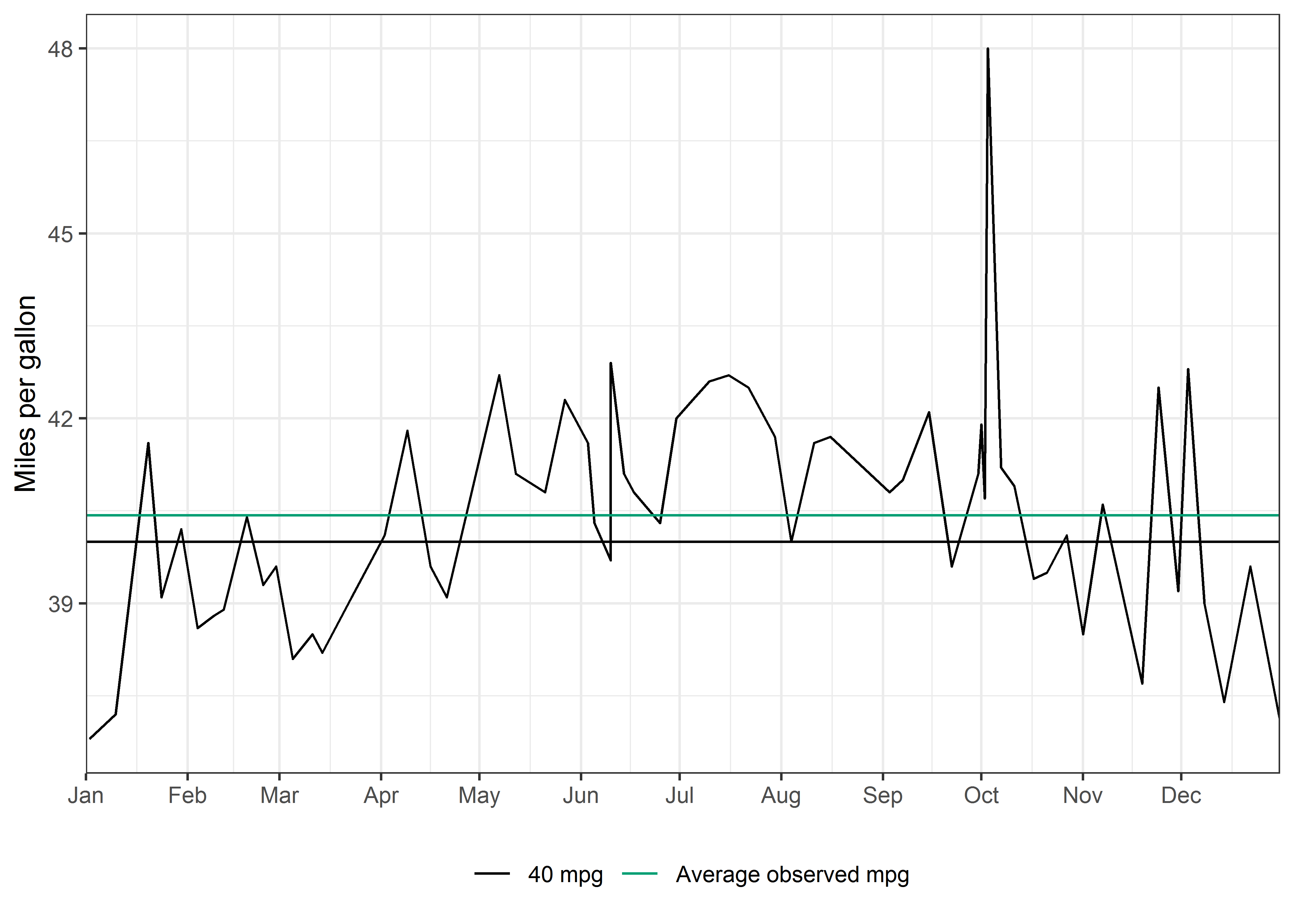

That high point is a high value for both the observed and estimated mpg, so I’m guessing the driving conditions were good for that tank. 😄

filter(fiesta2017, mpgcalc > 45)

## # A tibble: 1 x 6
##   date       gallons  cost mileage mpggage mpgcalc
##   <date>       <dbl> <dbl>   <dbl>   <dbl>   <dbl>
## 1 2017-10-03    8.37  25.6    401.    46.8      48

Compare observed mpg vs car-estimated mpg

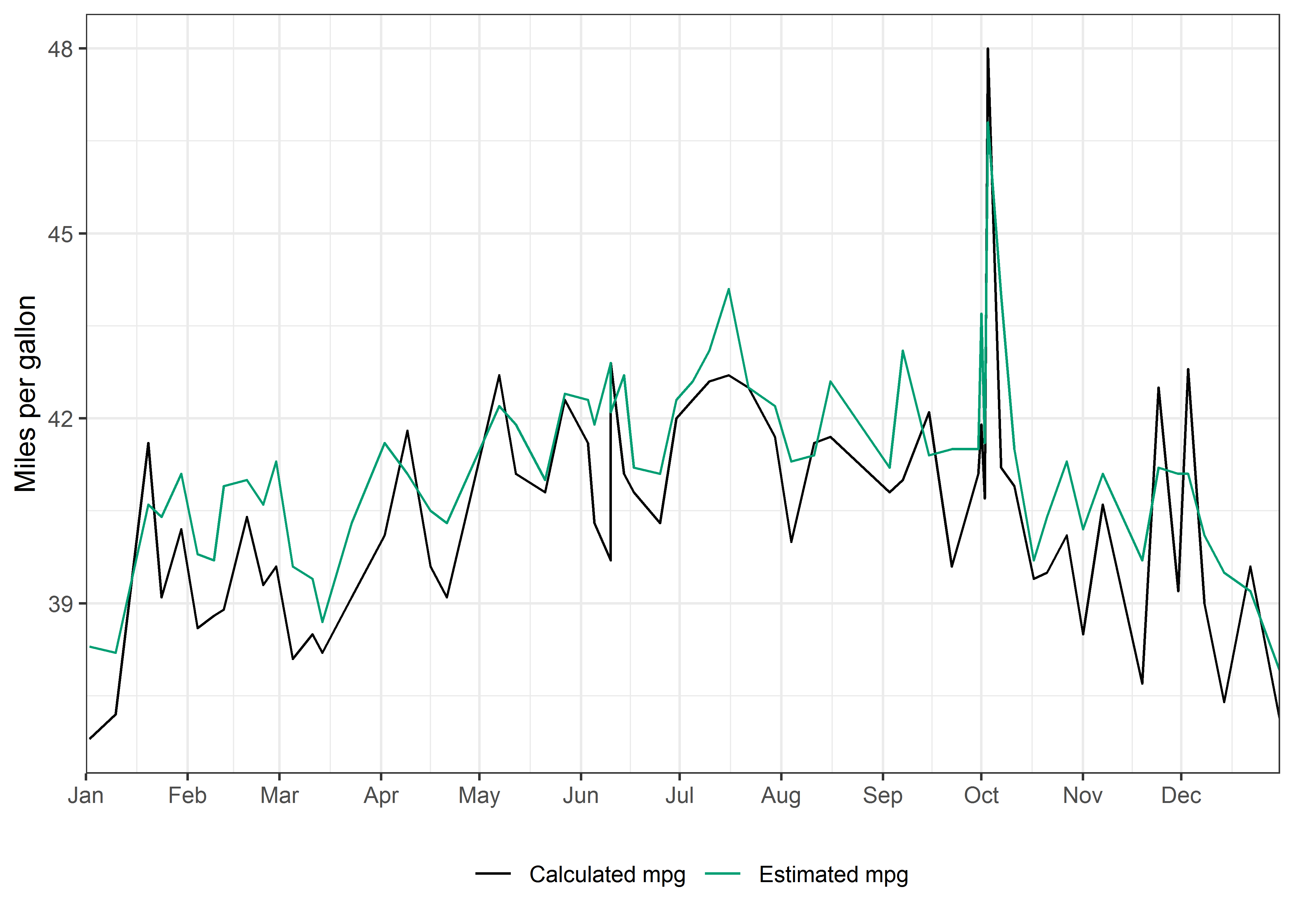
It’s fun to watch how the estimated mpg is affected by conditions while I’m driving (e.g., AC, defrost, wind), but it looks like whatever that algorithm is tends to overestimate the gas mileage. But not always!

ggplot(fiesta2017, aes(date, mpgcalc) ) +
     geom_line( aes(color = "Calculated mpg") ) +
     geom_line( aes(y = mpggage, color = "Estimated mpg") ) +
     theme_bw() +
     labs(y = "Miles per gallon", x = NULL) +
     scale_x_date(date_breaks = "1 month",
                  date_labels = "%b",
                  limits = c( as.Date("2017-01-01"), as.Date("2017-12-31") ),
                  expand = c(0, 0) ) +
     scale_color_manual(name = NULL, values = c("black", "#009E73") ) +
     theme(legend.position = "bottom",
           legend.direction = "horizontal")