Simulate! Simulate! - Part 1: A linear model
Confession: I love simulations.
I have found simulations incredibly useful in growing my understanding of statistical theory and assumptions of models. When someone tells me with great certainty “I don’t need to meet that assumption because [fill in the blank]” or asks “Does it matter that [something complicated]?”, I often turn to simulations instead of textbooks to check.
I like simulations for the same reasons I like building Bayesian models and using resampling methods (i.e., Monte Carlo) for inference. Building the simulation increases my understanding of the problem and makes all the assumptions clearer to me because I must define them explicitly. Plus I think it is fun to put the code together and explore the results. 🙂
Table of Contents
Simulate, simulate, dance to the music
Simulations have been so helpful in my own understanding of models used for analysis that I want to spread the knowledge. Being able to build a simulation can really help folks understand the strengths and weaknesses of their analysis. I haven’t managed to fit teaching simulations in my own work so far, but it’s always on my mind. Hence, this post.
Today I’m going to go over an example of simulating data from a two-group linear model. I’ll work work up to linear mixed models and generalized linear mixed models (the fun stuff! 😆) in subsequent posts.
The statistical model
Warning: Here there be equations.
If you’re like me and your brain says “I think this section must not pertain to me” when your eyes land on mathematical notation, you can jump right down to the R code in the next section. But if you can power through, I’ve found these equations are actually pretty useful when setting up a simulation (honest).
A simulation for a linear model is based on the statistical model. The statistical model is an equation that describes the processes we believe gave rise to the observed response variable. It includes parameters to describe the assumed effect of explanatory variables on the response variable as well as a description of any distributions associated with processes we assume are random variation. (There is more in-depth coverage of the statistical model in Stroup’s 2013 Generalized Linear Mixed Models book if you are interested and have access to it.)
The statistical model is where we write down the exact assumptions we are making when we fit a linear model to a set of data.
Here is an example of a linear model for two groups. I wrote the statistical model to match the form of the default summary output from a model fit with lm() in R.
\[y_t = \beta_0 + \beta_1*I_{(group_t=\textit{group2})} + \epsilon_t\]
- \(y_t\) is the observed values for the quantitative response variable; \(t\) goes from 1 to the number of observations in the dataset
- \(\beta_0\) is the mean response variable when the group is group1
- \(\beta_1\) is the difference in mean response between the two groups, group2 minus group1.
- The indicator variable, \(I_{(group_t=\textit{group2})}\), is 1 when the group is group2 and 0 otherwise, so \(\beta_1\) only affects the response variable for observations in group2
- \(\epsilon_t\) is the random variation present for each observation that is not explained by the group variable. These are assumed to come from an iid normal distribution with a mean of 0 and some shared variance, \(\sigma^2\): \(\epsilon_t \thicksim N(0, \sigma^2)\)
R packages
I’ll use package purrr for looping, broom for extracting output of models, dplyr for any data manipulation, and ggplot2 for plotting.
library(purrr) # v. 0.3.4
library(broom) # v. 0.5.6
library(dplyr) # v. 1.0.0
library(ggplot2) # v. 3.3.1
A single simulation from a two-group model
Let’s jump in and start simulating, as I find the statistical model becomes clearer once we have a simulated dataset to look at.
Here is what the dataset I will create will look like. I have a variable for the two groups (group) and one for the response variable (growth). There are 10 observations in each group.
#     group    growth
# 1  group1  5.952827
# 2  group1  4.749240
# 3  group1  7.192432
# 4  group1  2.111542
# 5  group1  7.295659
# 6  group1  4.063176
# 7  group1  2.988099
# 8  group1  5.127125
# 9  group1  7.049945
# 10 group1  6.146284
# 11 group2  6.694364
# 12 group2  3.223867
# 13 group2  1.507925
# 14 group2  6.316427
# 15 group2  4.443441
# 16 group2 -0.326161
# 17 group2  4.151819
# 18 group2  3.945520
# 19 group2  1.914537
# 20 group2  5.255374
I’ll set my seed so these particular results can be reproduced. I usually set the seed when I’m first working out my simulation process (but not when actually running the simulation many times).
set.seed(16)I start out by defining what the “truth” is in the simulation by setting all the parameters in the statistical model to a value of my choosing. Here’s what I’ll do today.
- The true group mean (\(\beta_0\)) for “group1” will be 5
- The mean of
group2will be 2 less thangroup1(\(\beta_1\)) - The shared variance (\(\sigma^2\)) will be set at 4, so the standard deviation (\(\sigma\)) is 2.
I’ll define the number of groups (2) and number of replicates per group (10) while I’m at it. The total number of observations is the number of groups times the number of replicates per group, 2*10 = 20.
ngroup = 2
nrep = 10
b0 = 5
b1 = -2
sd = 2
I need to create the variable I’ll call group to use as the explanatory variable when fitting a model in R. I use the function rep() a lot when doing simulations in order to repeat values of variables to appropriately match the scenario I’m building data for.
Here I’ll repeat each level of group 10 times (nrep as I defined above).
( group = rep( c("group1", "group2"), each = nrep) )# [1] "group1" "group1" "group1" "group1" "group1" "group1" "group1" "group1"
# [9] "group1" "group1" "group2" "group2" "group2" "group2" "group2" "group2"
# [17] "group2" "group2" "group2" "group2"Next I’ll simulate the random errors. Remember I defined these in the statistical model as \(\epsilon_t \thicksim N(0, \sigma^2)\). To simulate these I’ll take random draws from a normal distribution with a mean of 0 and standard deviation of 2. Note that rnorm() takes the standard deviation as input, not the variance.
Every observation (\(t\)) has a unique value for the random error, so I need to make 20 draws total (ngroup*nrep).
( eps = rnorm(n = ngroup*nrep, mean = 0, sd = sd) )# [1] 0.9528268 -0.2507600 2.1924324 -2.8884581 2.2956586 -0.9368241
# [7] -2.0119012 0.1271254 2.0499452 1.1462840 3.6943642 0.2238667
# [13] -1.4920746 3.3164273 1.4434411 -3.3261610 1.1518191 0.9455202
# [19] -1.0854633 2.2553741Now I have the fixed estimates of parameters, the variable group on which to base the indicator variable, and the random errors drawn from the defined distribution. That’s all the pieces I need to calculate my response variable.
The statistical model
\[y_t = \beta_0 + \beta_1*I_{(group_t=\textit{group2})} + \epsilon_t\]
is my guide for how to combine these pieces to create the simulated response variable, \(y_t\). Notice I create the indicator variable in R with group == "group2" and call the simulated response variable growth.
( growth = b0 + b1*(group == "group2") + eps )# [1] 5.952827 4.749240 7.192432 2.111542 7.295659 4.063176 2.988099
# [8] 5.127125 7.049945 6.146284 6.694364 3.223867 1.507925 6.316427
# [15] 4.443441 -0.326161 4.151819 3.945520 1.914537 5.255374I often store the variables I will use in fitting the model in a dataset to help keep things organized. This becomes more important when working with more variables.
dat = data.frame(group, growth)Once the response and explanatory variables have been created, it’s time to fit a model. I can fit the two group linear model with lm(). I call this test model growthfit.
growthfit = lm(growth ~ group, data = dat)
summary(growthfit)
#
# Call:
# lm(formula = growth ~ group, data = dat)
#
# Residuals:
# Min 1Q Median 3Q Max
# -4.039 -1.353 0.336 1.603 2.982
#
# Coefficients:
# Estimate Std. Error t value Pr(>|t|)
# (Intercept) 5.2676 0.6351 8.294 1.46e-07 ***
# groupgroup2 -1.5549 0.8982 -1.731 0.101
# ---
# Signif. codes: 0 '***' 0.001 '**' 0.01 '*' 0.05 '.' 0.1 ' ' 1
#
# Residual standard error: 2.008 on 18 degrees of freedom
# Multiple R-squared: 0.1427, Adjusted R-squared: 0.0951
# F-statistic: 2.997 on 1 and 18 DF, p-value: 0.1005Make a function for the simulation
A single simulation can help us understand the statistical model, but it doesn’t help us see how the model behaves over the long run. To repeat this simulation many times in R we’ll want to “functionize” the data simulating and model fitting process.
In my function I’m going to set all the arguments to the parameter values I’ve defined above. I allow some flexibility, though, so the argument values can be changed if I want to explore the simulation with different coefficient values, a different number of replications, or a different amount of random variation.
This function returns a linear model fit with lm().
twogroup_fun = function(nrep = 10, b0 = 5, b1 = -2, sigma = 2) {
     ngroup = 2
     group = rep( c("group1", "group2"), each = nrep)
     eps = rnorm(n = ngroup*nrep, mean = 0, sd = sigma)
     growth = b0 + b1*(group == "group2") + eps
     simdat = data.frame(group, growth)
     growthfit = lm(growth ~ group, data = simdat)
     growthfit
}
I test the function, using the same seed as I used figuring out the process to make sure things are working as expected. If things are working, I should get the same results as I did above. Looks good.
set.seed(16)
twogroup_fun()
#
# Call:
# lm(formula = growth ~ group, data = simdat)
#
# Coefficients:
# (Intercept) groupgroup2
# 5.268 -1.555If I want to change some element of the simulation, I can do so by changing the default values to the function arguments. Here’s a simulation from the same model but with a smaller standard deviation. All other arguments use the defaults I set.
twogroup_fun(sigma = 1)#
# Call:
# lm(formula = growth ~ group, data = simdat)
#
# Coefficients:
# (Intercept) groupgroup2
# 5.313 -2.476Repeat the simulation many times
Now that I have a working function to simulate data and fit the model, it’s time to do the simulation many times. I want to save the model from each individual simulation to allow exploration of long run model performance.
This is a task for the replicate() function, which repeatedly calls a function and saves the output. I use simplify = FALSE so the output is a list. This is convenient for going through to extract elements from the models later. Also see purrr::rerun() as a convenient version of replicate().
I’ll run this simulation 1000 times, resulting in a list of fitted two-group linear models based on data simulated from the parameters I’ve set set. I print the first model in the list below.
sims = replicate(n = 1000, twogroup_fun(), simplify = FALSE )
sims[[1]]
#
# Call:
# lm(formula = growth ~ group, data = simdat)
#
# Coefficients:
# (Intercept) groupgroup2
# 5.290 -1.463Extracting results from the linear model
There are many elements of our model that we might be interested in exploring, including estimated coefficients, estimated standard deviations/variances, and the statistical results (test statistics/p-values).
To get the coefficients and statistical tests of coefficients we can use tidy() from package broom.
This returns the information on coefficients and tests of those coefficients in a tidy format that is easy to work with. Here’s what the results look like for the test model.
tidy(growthfit)# # A tibble: 2 x 5
# term estimate std.error statistic p.value
# <chr> <dbl> <dbl> <dbl> <dbl>
# 1 (Intercept) 5.27 0.635 8.29 0.000000146
# 2 groupgroup2 -1.55 0.898 -1.73 0.101I have often been interested in understanding how the variances/standard deviations behave over the long run, in particular in mixed models. For a linear model we can extract an estimate of the residual standard deviation from the summary() output. This can be squared to get the variance as needed.
summary(growthfit)$sigma# [1] 2.008435Extract simulation results
Now for the fun part! Given we know the true model, how do the parameters behave over many samples?
To extract any results I’m interested in I will loop through the list of models, which I’ve stored in sims, and pull out the element of interest. I will use functions from the map family from package purrr for looping through the list of models. I’ll use functions from dplyr for any data manipulation and plot distributions via ggplot2.
Estimated differences in mean response
As this is a linear model about differences among the two groups, the estimate of \(\beta_1\) is one of the statistics of primary interest. What does the distribution of differences in mean growth between groups look like across the 1000 simulated datasets? Here’s a density plot.
sims %>%
     map_df(tidy) %>%
     filter(term == "groupgroup2") %>%
     ggplot( aes(x = estimate) ) +
          geom_density(fill = "blue", alpha = .5) +
          geom_vline( xintercept = -2)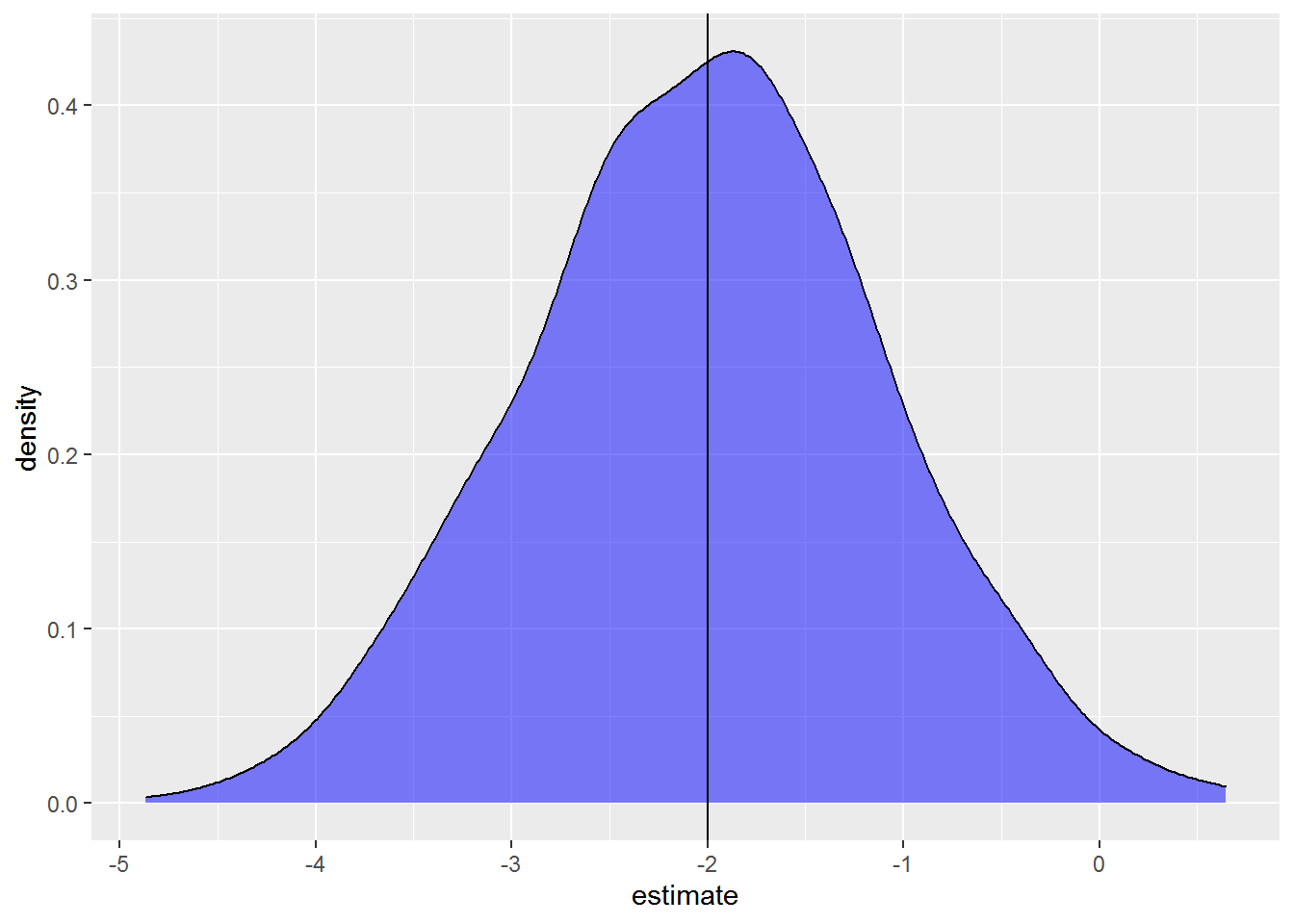
These are the kinds of results I find so compelling when doing simulations. The dataset I made is pretty small and has a fair amount of unexplained variation. While on average we get the correct result, since the peak of the distribution is right around the true value of -2, there is quite a range in the estimated coefficient across simulations. Some samples lead to overestimates and some to underestimates of the parameter. Some models even get the sign of the coefficient wrong. If we had only a single model from a single sample, as we would when collecting data rather than simulating data, we could very well get a fairly bad estimate for the value we are interested in.
See Gelman and Carlin’s 2014 paper, Beyond Power Calculations: Assessing Type S (Sign) and Type M (Magnitude) Errors if you are interested in further discussion.
Estimated standard deviation
I can do a similar plot exploring estimates of the residual standard deviation. In this case I extract sigma from the model object and put it in a data.frame to plot the distribution with a density plot.
sims %>%
     map_dbl(~summary(.x)$sigma) %>%
     data.frame(sigma = .) %>%
     ggplot( aes(x = sigma) ) +
          geom_density(fill = "blue", alpha = .5) +
          geom_vline(xintercept = 2)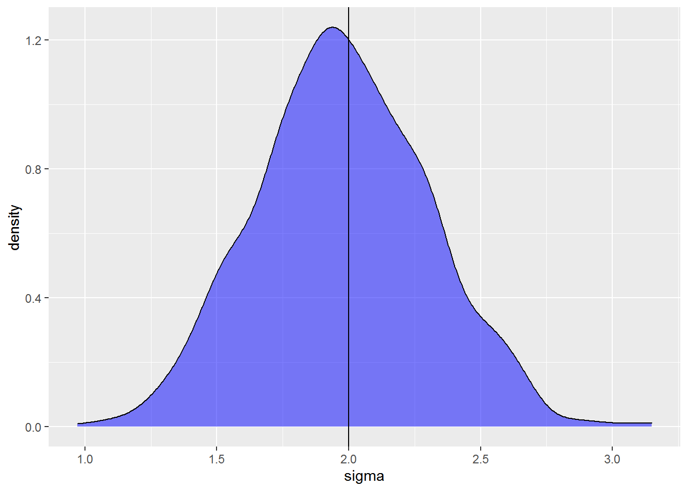
The estimated variation ranges between 1 to just over 3, and the distribution is roughly centered on the true value of 2. Like with the coefficient above, the model performs pretty well on average but any single model can have a biased estimate of the standard deviation.
The standard deviation is underestimated a bit more than 50% of the time. This is not uncommon.
sims %>%
     map_dbl(~summary(.x)$sigma) %>%
     {. < 2} %>%
     mean()
# [1] 0.539Extract hypothesis test results
If the goal of a simulation is to get an idea of the statistical power of a test we could look at the proportion of times the null hypothesis was rejected given a fixed alpha level (often 0.05, but of course it can be something else).
Here the proportion of models that correctly rejected the null hypothesis, given that we know the null hypothesis is not true, is just over 56%. That’s an estimate of the statistical power.
sims %>%
     map_df(tidy) %>%
     filter(term == "groupgroup2") %>%
     pull(p.value) %>%
     {. <  0.05} %>%
     mean()
# [1] 0.563The three examples I gave above are common statistics of interest but really any output from the model is fair game. For linear models you could also pull out \(R^2\) or the overall F-test, for example.
Where to go from here?
I’ll do future posts about simulating from more complicated linear models, starting with linear mixed models. In particular I will explore interesting issues that crop up when estimating variances in part 2 of the series.
Just the code, please
Here’s the code without all the discussion. Copy and paste the code below or you can download an R script of uncommented code from here.
library(purrr) # v. 0.3.4
library(broom) # v. 0.5.6
library(dplyr) # v. 1.0.0
library(ggplot2) # v. 3.3.1

dat
set.seed(16)
ngroup = 2
nrep = 10
b0 = 5
b1 = -2
sd = 2

( group = rep( c("group1", "group2"), each = nrep) )
( eps = rnorm(n = ngroup*nrep, mean = 0, sd = sd) )
( growth = b0 + b1*(group == "group2") + eps )

dat = data.frame(group, growth)

growthfit = lm(growth ~ group, data = dat)
summary(growthfit)

twogroup_fun = function(nrep = 10, b0 = 5, b1 = -2, sigma = 2) {
     ngroup = 2
     group = rep( c("group1", "group2"), each = nrep)
     eps = rnorm(n = ngroup*nrep, mean = 0, sd = sigma)
     growth = b0 + b1*(group == "group2") + eps
     simdat = data.frame(group, growth)
     growthfit = lm(growth ~ group, data = simdat)
     growthfit
}

set.seed(16)
twogroup_fun()

twogroup_fun(sigma = 1)

sims = replicate(n = 1000, twogroup_fun(), simplify = FALSE )
sims[[1]]

tidy(growthfit)

summary(growthfit)$sigma

sims %>%
     map_df(tidy) %>%
     filter(term == "groupgroup2") %>%
     ggplot( aes(x = estimate) ) +
          geom_density(fill = "blue", alpha = .5) +
          geom_vline( xintercept = -2)

sims %>%
     map_dbl(~summary(.x)$sigma) %>%
     data.frame(sigma = .) %>%
     ggplot( aes(x = sigma) ) +
          geom_density(fill = "blue", alpha = .5) +
          geom_vline(xintercept = 2)

sims %>%
     map_dbl(~summary(.x)$sigma) %>%
     {. < 2} %>%
     mean()

sims %>%
     map_df(tidy) %>%
     filter(term == "groupgroup2") %>%
     pull(p.value) %>%
     {. <  0.05} %>%
     mean()