Simulate! Simulate! - Part 2: A linear mixed model
This post was last updated on 2021-12-21.
I feel like I learn something every time start simulating new data to update an assignment or exploring a question from a client via simulation. I’ve seen instances where residual autocorrelation isn’t detectable when I know it exists (because I simulated it) or I have skewed residuals and/or unequal variances when I simulated residuals from a normal distribution with a single variance. Such results are often due to small sample sizes, which even in this era of big data still isn’t so unusual in ecology. I’ve found exploring the effect of sample size on statistical results to be quite eye-opening 👁.
In my first simulation post I showed how to simulate data for a basic linear model. Today I’ll be talking about how to simulate data for a linear mixed model. So I’m still working with normally distributed residuals but will add an additional level of variation.
Table of Contents
- Simulate, simulate, dance to the music
- The statistical model
- A single simulation for the two-level model
- Make a function for the simulation
- Repeat the simulation many times
- Extract results from the linear mixed model
- Explore the effect of sample size on variance estimation
- An actual mixed model (with fixed effects this time)
- Just the code, please
Simulate, simulate, dance to the music
I learned the basics of linear mixed models in a class where we learned how to analyze data from “classically designed” experiments. We spent a lot of time writing down the various statistical models in mathematical notation and then fitting said models in SAS. I felt like I understood the basics of mixed models when the class was over (and swore I was done with all the \(i\) and \(j\) mathematical notation once and for all 😆).
It wasn’t until I started working with clients and teaching labs on mixed models in R that I learned how to do simulations to understand how well such models worked under various scenarios. These simulations took me to a whole new level of understanding of these models and the meaning of all that pesky mathematical notation.
The statistical model
Danger, equations below!
You can opt to jump to the next section if you don’t find equations useful.
If you don’t have a good understanding of the statistical model (or even if you do), writing it out in mathematical notation can actually be pretty useful. I’ll write a relatively simple model with random effects below. (Note that I only have an overall mean in this model; I’ll do a short example at the end of the post to show how one can simulate additional fixed effects.)
The study design that is the basis of my model has two different sizes of study units. I’m using a classic forestry example, where stands of trees are somehow chosen for sampling and then multiple plots within each stand are measured. This is a design with two levels, stands and plots; we could add a third level if individual trees were measured in each plot.
Everything today will be perfectly balanced, so the same number of plots will be sampled in each stand.
I’m using (somewhat sloppy) “regression” style notation instead of experimental design notation, where the \(t\) indexes the observations.
\[y_t = \mu + (b_s)_t + \epsilon_t\]
- \(y_t\) is the recorded value for the \(t\)th observation of the quantitative response variable; \(t\) goes from 1 to the number of observations in the dataset. Since plot is the level of observation in this example (i.e., we have a single observation for each plot), \(t\) indexes both the number of plots and the number of rows in the dataset.
- \(\mu\) is the overall mean response
- \(b_s\) is the (random) effect of the \(s\)th stand on the response. \(s\) goes from 1 to the total number of stands sampled. The stand-level random effects are assumed to come from an iid normal distribution with a mean of 0 and some shared, stand-level variance, \(\sigma^2_s\): \(b_s \thicksim N(0, \sigma^2_s)\)
- \(\epsilon_t\) is the observation-level random effect (the residual error term). Since plots are the level of observation in my scenario, this is essentially the effect of each plot measurement on the response. These are assumed to come from an iid normal distribution with a mean of 0 and some shared variance, \(\sigma^2\): \(\epsilon_t \thicksim N(0, \sigma^2)\)
A single simulation for the two-level model
Let’s jump in and start simulating, as I find the statistical model becomes clearer once we have a simulated dataset to look at.
Here is what the dataset I will create will look like. I have a variable for stands (stand), plots (plot), and the response variable (resp).
#    stand plot      resp
# 1      A    a 10.484415
# 2      A    b  9.946876
# 3      A    c 11.016389
# 4      A    d 11.977799
# 5      B    e 10.322382
# 6      B    f 11.596422
# 7      B    g  9.861173
# 8      B    h  9.003203
# 9      C    i 13.850646
# 10     C    j 12.914153
# 11     C    k 10.529352
# 12     C    l 12.768342
# 13     D    m  7.584302
# 14     D    n  6.568810
# 15     D    o  8.239229
# 16     D    p  5.463744
# 17     E    q 11.981485
# 18     E    r 12.112977
# 19     E    s 13.766137
# 20     E    t 11.429760
I’ll start by setting the seed so these results can be exactly reproduced.
set.seed(16)I need to define the “truth” in the simulation by setting all the parameters in the statistical model to a value of my choosing. Here’s what I’ll do today.
- The true mean (\(\mu\)) will be 10
- The stand-level variance (\(\sigma^2_s\)) will be set at 4, so the standard deviation (\(\sigma_s\)) is 2.
- The observation-level random effect variance (\(\sigma^2\)) will be set at 1, so the standard deviation (\(\sigma\)) is 1.
I’ll define the number of groups and number of replicates per group while I’m at it. I’ll use 5 stands and 4 plots per stand. The total number of plots (and so observations) is the number of stands times the number of plots per stand: 5*4 = 20.
nstand = 5
nplot = 4
mu = 10
sds = 2
sd = 1
I need to create a stand variable, containing unique names for the five sampled stands. I use capital letters for this. Each stand name will be repeated four times, because each one was measured four times (i.e., there are four plots in each stand).
( stand = rep(LETTERS[1:nstand], each = nplot) )# [1] "A" "A" "A" "A" "B" "B" "B" "B" "C" "C" "C" "C" "D" "D" "D" "D" "E" "E" "E"
# [20] "E"I can make a plot variable, as well, although it’s not needed for modeling since we have a single value per plot. It is fairly common to give plots the same name in each stand (i.e., plots are named 1-4 in each stand), but I’m a big believer in giving plots unique names. I’ll name plots uniquely using lowercase letters. There are a total of 20 plots.
( plot = letters[1:(nstand*nplot)] )# [1] "a" "b" "c" "d" "e" "f" "g" "h" "i" "j" "k" "l" "m" "n" "o" "p" "q" "r" "s"
# [20] "t"Now I will simulate the stand-level random effects. I defined these as \(b_s \thicksim N(0, \sigma^2_s)\), so will randomly draw from a normal distribution with a mean of 0 and standard deviation of 2 (remember that rnorm() in R uses standard deviation, not variance). I have five stands, so I draw five values.
( standeff = rnorm(nstand, 0, sds) )# [1] 0.9528268 -0.2507600 2.1924324 -2.8884581 2.2956586Every plot in a stand has the same “stand effect”, which I simulated with the five values above. This means that the stand itself is causing the measured response variable to be higher or lower than other stands across all plots in the stand. So the “stand effect” must be repeated for every plot in a stand.
The stand variable I made helps me know how to repeat the stand effect values. Based on that variable, every stand effect needs to be repeated four times in a row (once for each plot).
( standeff = rep(standeff, each = nplot) )# [1] 0.9528268 0.9528268 0.9528268 0.9528268 -0.2507600 -0.2507600
# [7] -0.2507600 -0.2507600 2.1924324 2.1924324 2.1924324 2.1924324
# [13] -2.8884581 -2.8884581 -2.8884581 -2.8884581 2.2956586 2.2956586
# [19] 2.2956586 2.2956586The observation-level random effect is simulated the same way as for a linear model. Every unique plot measurement has some effect on the response, and that effect is drawn from a normal distribution with a mean of 0 and a standard deviation of 1 (\(\epsilon_t \thicksim N(0, \sigma^2)\)).
I make 20 draws from this distribution, one for every plot/observation.
( ploteff = rnorm(nstand*nplot, 0, sd) )# [1] -0.46841204 -1.00595059 0.06356268 1.02497260 0.57314202 1.84718210
# [7] 0.11193337 -0.74603732 1.65821366 0.72172057 -1.66308050 0.57590953
# [13] 0.47276012 -0.54273166 1.12768707 -1.64779762 -0.31417395 -0.18268157
# [19] 1.47047849 -0.86589878I’m going to put all of these variables in a dataset together. This helps me keep things organized for modeling but, more importantly for learning how to do simulations, I think this helps demonstrate how every stand has an overall effect (repeated for every observation in that stand) and every plot has a unique effect. This becomes clear when you peruse the 20-row dataset shown below.
( dat = data.frame(stand, standeff, plot, ploteff) )# stand standeff plot ploteff
# 1 A 0.9528268 a -0.46841204
# 2 A 0.9528268 b -1.00595059
# 3 A 0.9528268 c 0.06356268
# 4 A 0.9528268 d 1.02497260
# 5 B -0.2507600 e 0.57314202
# 6 B -0.2507600 f 1.84718210
# 7 B -0.2507600 g 0.11193337
# 8 B -0.2507600 h -0.74603732
# 9 C 2.1924324 i 1.65821366
# 10 C 2.1924324 j 0.72172057
# 11 C 2.1924324 k -1.66308050
# 12 C 2.1924324 l 0.57590953
# 13 D -2.8884581 m 0.47276012
# 14 D -2.8884581 n -0.54273166
# 15 D -2.8884581 o 1.12768707
# 16 D -2.8884581 p -1.64779762
# 17 E 2.2956586 q -0.31417395
# 18 E 2.2956586 r -0.18268157
# 19 E 2.2956586 s 1.47047849
# 20 E 2.2956586 t -0.86589878I now have the fixed values of the parameters, the variable stand to represent the random effect in a model, and the simulated effects of stands and plots drawn from their defined distributions. That’s all the pieces I need to calculate my response variable.
The statistical model
\[y_t = \mu + (b_s)_t + \epsilon_t\]
is my guide for how to combine these pieces to create the simulated response variable, \(y_t\). Notice I call the simulated response variable resp.
( dat$resp = with(dat, mu + standeff + ploteff ) )# [1] 10.484415 9.946876 11.016389 11.977799 10.322382 11.596422 9.861173
# [8] 9.003203 13.850646 12.914153 10.529352 12.768342 7.584302 6.568810
# [15] 8.239229 5.463744 11.981485 12.112977 13.766137 11.429760Now that I have successfully created the dataset I showed you at the start of this section, it’s time for model fitting! I can fit a model with two sources of variation (stand and plot) with, e.g., the lmer() function from package lme4.
library(lme4) # v. 1.1-27.1The results for the estimated overall mean and standard deviations of random effects in this model look pretty similar to my defined parameter values.
fit1 = lmer(resp ~ 1 + (1|stand), data = dat)
fit1
# Linear mixed model fit by REML ['lmerMod']
# Formula: resp ~ 1 + (1 | stand)
# Data: dat
# REML criterion at convergence: 72.5943
# Random effects:
# Groups Name Std.Dev.
# stand (Intercept) 2.168
# Residual 1.130
# Number of obs: 20, groups: stand, 5
# Fixed Effects:
# (Intercept)
# 10.57Make a function for the simulation
A single simulation can help us understand the statistical model, but usually the goal of a simulation is to see how the model behaves over the long run. To repeat this simulation many times in R we’ll want to “functionize” the data simulating and model fitting process.
In my function I’m going to set all the arguments to the parameter values as I defined them above. I allow some flexibility, though, so the argument values can be changed if I want to explore the simulation with, say, a different number of replications or different standard deviations at either level.
This function returns a linear model fit with lmer().
twolevel_fun = function(nstand = 5, nplot = 4, mu = 10, sigma_s = 2, sigma = 1) {
     standeff = rep( rnorm(nstand, 0, sigma_s), each = nplot)
     stand = rep(LETTERS[1:nstand], each = nplot)
     ploteff = rnorm(nstand*nplot, 0, sigma)
     resp = mu + standeff + ploteff
     dat = data.frame(stand, resp)
     lmer(resp ~ 1 + (1|stand), data = dat)
}
I test the function, using the same seed, to make sure things are working as expected and that I get the same results as above.
set.seed(16)
twolevel_fun()
# Linear mixed model fit by REML ['lmerMod']
# Formula: resp ~ 1 + (1 | stand)
# Data: dat
# REML criterion at convergence: 72.5943
# Random effects:
# Groups Name Std.Dev.
# stand (Intercept) 2.168
# Residual 1.130
# Number of obs: 20, groups: stand, 5
# Fixed Effects:
# (Intercept)
# 10.57Repeat the simulation many times
Now that I have a working function to simulate data and fit the model it’s time to do the simulation many times. The model from each individual simulation is saved to allow exploration of long run model performance.
This is a task for replicate(), which repeatedly calls a function and saves the output. When using simplify = FALSE the output is a list, which is convenient for going through to extract elements from the models later. I’ll re-run the simulation 100 times as an example, although I will do 1000 runs later when I explore the long-run performance of variance estimates.
sims = replicate(100, twolevel_fun(), simplify = FALSE )
sims[[100]]
# Linear mixed model fit by REML ['lmerMod']
# Formula: resp ~ 1 + (1 | stand)
# Data: dat
# REML criterion at convergence: 58.0201
# Random effects:
# Groups Name Std.Dev.
# stand (Intercept) 1.7197
# Residual 0.7418
# Number of obs: 20, groups: stand, 5
# Fixed Effects:
# (Intercept)
# 7.711Extract results from the linear mixed model
After running all the models we will want to extract whatever we are interested in. The tidy() function from package broom.mixed can be used to conveniently extract both fixed and random effects.
Below is an example on the practice model. You’ll notice there are no p-values for fixed effects. If those are desired and the degrees of freedom can be calculated, see packages lmerTest and the ddf.method argument in tidy().
library(broom.mixed) # v. 0.2.7
tidy(fit1)
# # A tibble: 3 x 6
# effect group term estimate std.error statistic
# <chr> <chr> <chr> <dbl> <dbl> <dbl>
# 1 fixed <NA> (Intercept) 10.6 1.00 10.5
# 2 ran_pars stand sd__(Intercept) 2.17 NA NA
# 3 ran_pars Residual sd__Observation 1.13 NA NAIf we want to extract only the fixed effects:
tidy(fit1, effects = "fixed")# # A tibble: 1 x 5
# effect term estimate std.error statistic
# <chr> <chr> <dbl> <dbl> <dbl>
# 1 fixed (Intercept) 10.6 1.00 10.5And for the random effects, which can be pulled out as variances via scales instead of the default standard deviations:
tidy(fit1, effects = "ran_pars", scales = "vcov")# # A tibble: 2 x 4
# effect group term estimate
# <chr> <chr> <chr> <dbl>
# 1 ran_pars stand var__(Intercept) 4.70
# 2 ran_pars Residual var__Observation 1.28Explore the effect of sample size on variance estimation
Today I’ll look at how well we estimate variances of random effects for different samples sizes. I’ll simulate data for sampling 5 stands, 20 stands, and 100 stands.
I’m going to load some helper packages for this, including purrr for looping, dplyr for data manipulation tasks, and ggplot2 for plotting.
library(purrr) # v. 0.3.4
suppressPackageStartupMessages( library(dplyr) ) # v. 1.0.7
library(ggplot2) # v. 3.3.5
I’m going to loop through a vector of the three stand sample sizes and then simulate data and fit a model 1000 times for each one. I’m using purrr functions for this, and I end up with a list of lists (1000 models for each sample size). It takes a minute or two to fit the 3000 models. I’m ignoring all warning messages (but this isn’t always a good idea).
stand_sims = c(5, 20, 100) %>%
     set_names() %>%
     map(~replicate(1000, twolevel_fun(nstand = .x) ) )
Next I’ll pull out the stand variance for each model via tidy().
I use modify_depth() to work on the nested (innermost) list, and then row bind the nested lists into a data.frame to get things in a convenient format for plotting. I finish by filtering things to keep only the stand variance, as I extracted both stand and residual variances from the model.
stand_vars = stand_sims %>%
     modify_depth(2, ~tidy(.x, effects = "ran_pars", scales = "vcov") ) %>%
     map_dfr(bind_rows, .id = "stand_num") %>%
     filter(group == "stand")
head(stand_vars)
# # A tibble: 6 x 5
# stand_num effect group term estimate
# <chr> <chr> <chr> <chr> <dbl>
# 1 5 ran_pars stand var__(Intercept) 2.53
# 2 5 ran_pars stand var__(Intercept) 7.70
# 3 5 ran_pars stand var__(Intercept) 4.19
# 4 5 ran_pars stand var__(Intercept) 3.28
# 5 5 ran_pars stand var__(Intercept) 12.9
# 6 5 ran_pars stand var__(Intercept) 4.62Let’s take a look at the distributions of the variances for each sample size via density plots. We know the true variance is 4, so I’ll add a vertical line at 4.
ggplot(stand_vars, aes(x = estimate) ) +
     geom_density(fill = "blue", alpha = .25) +
     facet_wrap(~stand_num) +
     geom_vline(xintercept = 4)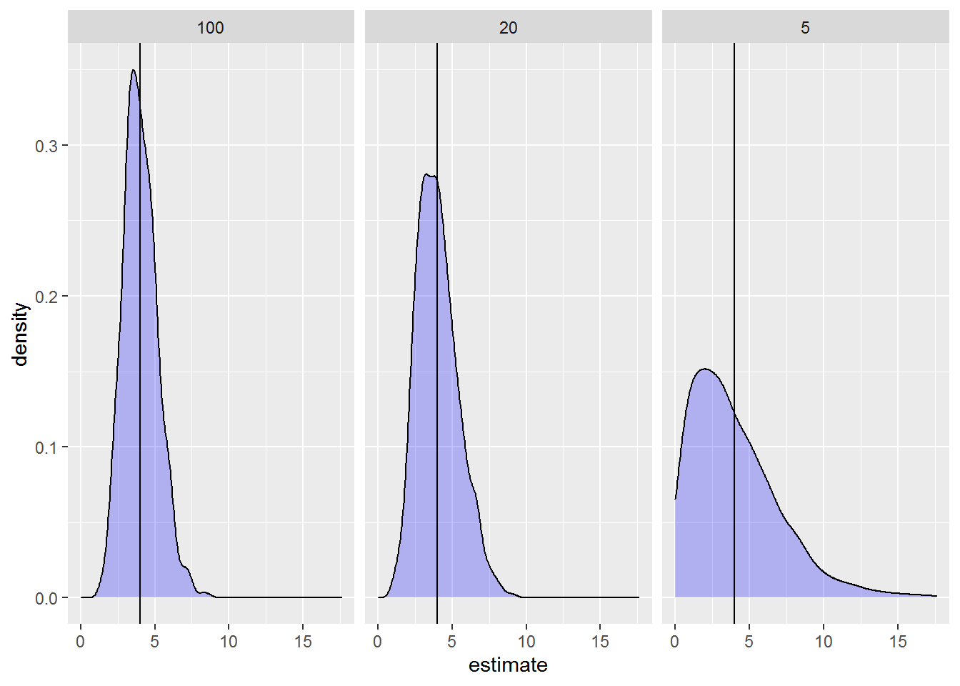
Whoops, I need to get my factor levels in order. I’ll use package forcats for this.
stand_vars = mutate(stand_vars, stand_num = forcats::fct_inorder(stand_num) )I’ll also add some clearer labels for the facets.
add_prefix = function(string) {
     paste("Number stands:", string, sep = " ")
}
And finally I’ll add the median of each distribution as a second vertical line.
groupmed = stand_vars %>%
     group_by(stand_num) %>%
     summarise(mvar = median(estimate) )
Looking at the plots we can really see how poorly we can estimate variances when we have few replications. When only 5 stands are sampled, the variance can be estimated as low as 0 and as high as ~18 (😮) when it’s really 4.
By the time we have 20 stands things look better, and things look quite good with 100 stands (although notice variance still ranges from 1 to ~8).
ggplot(stand_vars, aes(x = estimate) ) +
     geom_density(fill = "blue", alpha = .25) +
     facet_wrap(~stand_num, labeller = as_labeller(add_prefix) ) +
     geom_vline(aes(xintercept = 4, linetype = "True variance"), size = .5 ) +
     geom_vline(data = groupmed, aes(xintercept = mvar, linetype = "Median variance"),
                size = .5) +
     theme_bw(base_size = 14) +
     scale_linetype_manual(name = "", values = c(2, 1) ) +
     theme(legend.position = "bottom",
           legend.key.width = unit(.1, "cm") ) +
     labs(x = "Estimated Variance", y = NULL)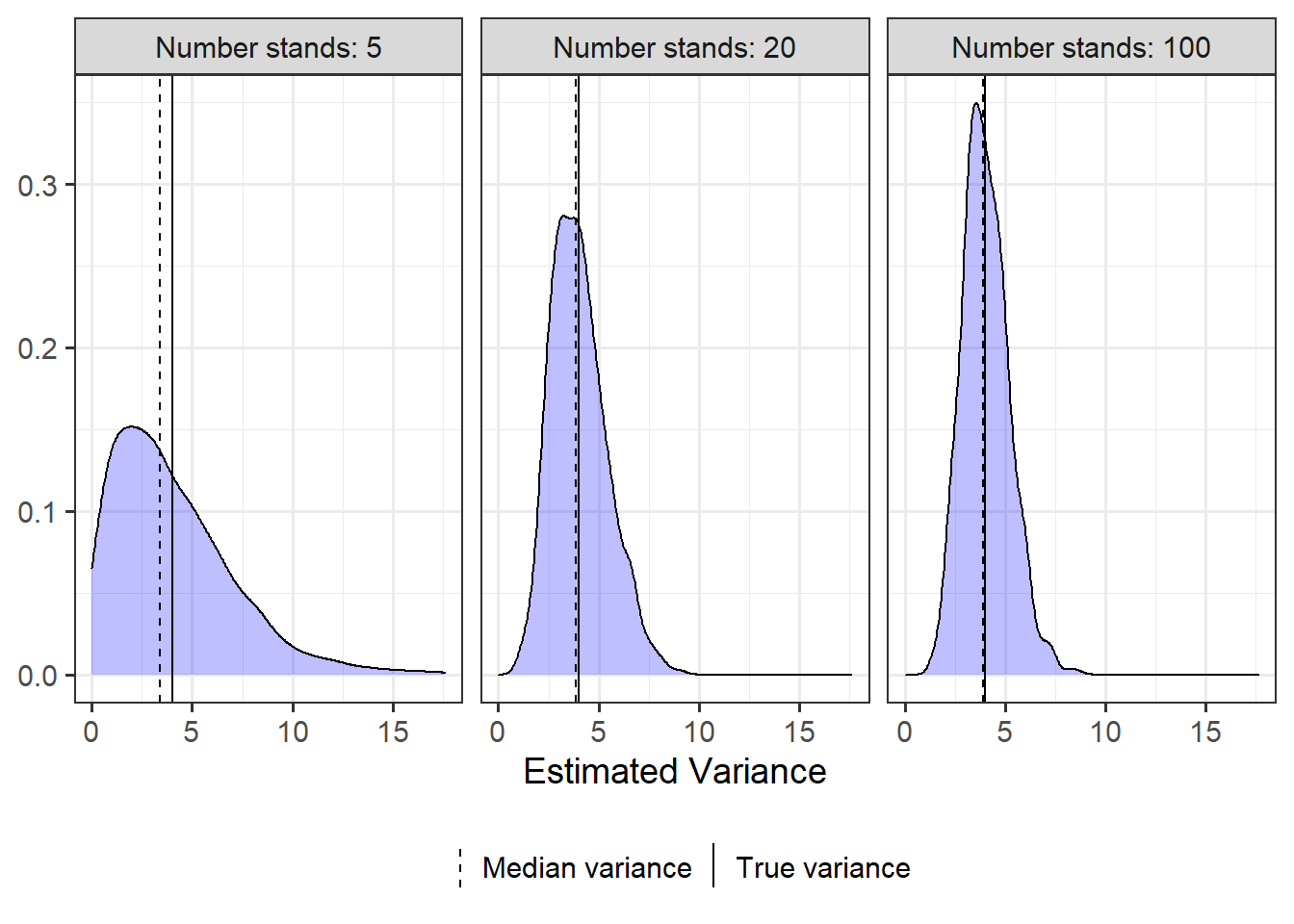
Here are some additional descriptive statistics of the distribution of variances in each group to complement the info in the plot.
stand_vars %>%
     group_by(stand_num) %>%
     summarise_at("estimate",
                  list(min = min, mean = mean, med = median, max = max) )
# # A tibble: 3 x 5
# stand_num min mean med max
# <fct> <dbl> <dbl> <dbl> <dbl>
# 1 5 0 4.04 3.39 17.6
# 2 20 0.994 4.03 3.88 9.15
# 3 100 1.27 4.04 3.92 8.71So how much of the distribution is below 4 for each estimate?
We can see for 5 samples that the variance is definitely underestimated more often than it is overestimated; almost 60% of the distribution is below the true variance of 4.
Every time I do this sort of simulation I am newly surprised that even large samples tend to underestimate variances slightly more often than overestimate them.
stand_vars %>%
     group_by(stand_num) %>%
     summarise(mean(estimate < 4) )
# # A tibble: 3 x 2
# stand_num `mean(estimate < 4)`
# <fct> <dbl>
# 1 5 0.577
# 2 20 0.532
# 3 100 0.525My take home from all of this? We may need to be cautious with results for studies where the goal is to make inference about the estimates of the variances or for testing variables measured at the level of the largest unit when the number of units is small.
An actual mixed model (with fixed effects this time)
I simplified things above so much that I didn’t have any fixed effects variables. We can certainly include fixed effects in a simulation.
Below is a quick example. I’ll create two continuous variables, one measured at the stand level and one measured at the plot level, that have linear relationships with the mean response variable. The study is the same as the one I defined for the previous simulation.
Here’s the new statistical model.
\[y_t = \beta_0 + \beta_1*(Elevation_s)_t + \beta_2*Slope_t + (b_s)_t + \epsilon_t\]
Where
- \(\beta_0\) is the mean response when both Elevation and Slope are 0
- \(\beta_1\) is the change in mean response for a 1-unit change in elevation. Elevation is measured at the stand level, so all plots in a stand share a single value of elevation.
- \(\beta_2\) is the change in mean response for a 1-unit change in slope. Slope is measured at the plot level, so every plot potentially has a unique value of slope.
Setting the values for the three new parameters and simulating values for the continuous explanatory variables will be additional steps in the simulation. The random effects are simulated the same way as before.
I define the new parameters below.
- The intercept (\(\beta_0\)) will be -1
- The coefficient for elevation (\(\beta_1\)) will be set to 0.005
- The coefficient for slope (\(\beta_2\)) will be set to 0.1
nstand = 5
nplot = 4
b0 = -1
b1 = .005
b2 = .1
sds = 2
sd = 1
Here are the variables I simulated previously.
set.seed(16)
stand = rep(LETTERS[1:nstand], each = nplot)
standeff = rep( rnorm(nstand, 0, sds), each = nplot)
ploteff = rnorm(nstand*nplot, 0, sd)
I will simulate the explanatory variables by randomly drawing from uniform distributions via runif(). I change the minimum and maximum values of the uniform distribution as needed to get an appropriate spread for a given variable. If the distribution of your explanatory variables are more skewed you could use a different distribution (like the Gamma distribution).
First I simulate values for elevation. This variable only five values, as it is a stand-level variable. I need to repeat each value for the four plots measured in each stand like I did when making the stand variable.
( elevation = rep( runif(nstand, 1000, 1500), each = nplot) )# [1] 1468.339 1468.339 1468.339 1468.339 1271.581 1271.581 1271.581 1271.581
# [9] 1427.050 1427.050 1427.050 1427.050 1166.014 1166.014 1166.014 1166.014
# [17] 1424.256 1424.256 1424.256 1424.256I can simulate slope the same way, pulling random values from a uniform distribution with different limits. The slope is measured at the plot level, so I have one value for every plot in the dataset.
( slope = runif(nstand*nplot, 2, 75) )# [1] 48.45477 60.37014 59.58588 44.76939 61.88313 20.29559 71.51617 42.35035
# [9] 63.67044 36.43613 10.58778 14.62304 35.11192 13.19697 9.29946 46.56462
# [17] 34.68245 53.61456 37.00606 42.30044We now have everything we need to create the response variable.
Based on our equation \[y_t = \beta_0 + \beta_1*(Elevation_s)_t + \beta_2*Slope_t + (b_s)_t + \epsilon_t\]
the response variable will be calculated via
( resp2 = b0 + b1*elevation + b2*slope + standeff + ploteff )# [1] 11.671585 12.325584 13.316671 12.796432 11.868602 8.983889 12.370697
# [8] 8.596145 16.352939 12.693014 7.723378 10.365894 5.925563 2.718576
# [15] 3.999244 4.950275 11.571009 13.595712 13.588022 11.781083Now we can fit a mixed model for resp2 with elevation and slope as fixed effects, stand as the random effect and the residual error term based on plot-to-plot variation. (Notice I didn’t put these variables in a dataset, which I usually like to do to keep things organized and to avoid problems of vectors in my environment getting overwritten by mistake.)
We can see some of the estimates in this one model aren’t very similar to our set values, and doing a full simulation would allow us to explore the variation in the estimates. For example, I expect the coefficient for elevation, based on only five values, will be extremely unstable.
lmer(resp2 ~ elevation + slope + (1|stand) )# Linear mixed model fit by REML ['lmerMod']
# Formula: resp2 ~ elevation + slope + (1 | stand)
# REML criterion at convergence: 81.9874
# Random effects:
# Groups Name Std.Dev.
# stand (Intercept) 1.099
# Residual 1.165
# Number of obs: 20, groups: stand, 5
# Fixed Effects:
# (Intercept) elevation slope
# -21.31463 0.02060 0.09511Just the code, please
Here’s the code without all the discussion. Copy and paste the code below or you can download an R script of uncommented code from here.
set.seed(16)
nstand = 5
nplot = 4
mu = 10
sds = 2
sd = 1

( stand = rep(LETTERS[1:nstand], each = nplot) )
( plot = letters[1:(nstand*nplot)] )
( standeff = rnorm(nstand, 0, sds) )
( standeff = rep(standeff, each = nplot) )
( ploteff = rnorm(nstand*nplot, 0, sd) )

( dat = data.frame(stand, standeff, plot, ploteff) )

( dat$resp = with(dat, mu + standeff + ploteff ) )

library(lme4) # v. 1.1-27.1

fit1 = lmer(resp ~ 1 + (1|stand), data = dat)
fit1

twolevel_fun = function(nstand = 5, nplot = 4, mu = 10, sigma_s = 2, sigma = 1) {
     standeff = rep( rnorm(nstand, 0, sigma_s), each = nplot)
     stand = rep(LETTERS[1:nstand], each = nplot)
     ploteff = rnorm(nstand*nplot, 0, sigma)
     resp = mu + standeff + ploteff
     dat = data.frame(stand, resp)
     lmer(resp ~ 1 + (1|stand), data = dat)
}

set.seed(16)
twolevel_fun()

sims = replicate(100, twolevel_fun(), simplify = FALSE )
sims[[100]]

library(broom.mixed) # v. 0.2.7
tidy(fit1)

tidy(fit1, effects = "fixed")

tidy(fit1, effects = "ran_pars", scales = "vcov")

library(purrr) # v. 0.3.4
suppressPackageStartupMessages( library(dplyr) ) # v. 1.0.7
library(ggplot2) # v. 3.3.5

stand_sims = c(5, 20, 100) %>%
     set_names() %>%
     map(~replicate(1000, twolevel_fun(nstand = .x) ) )

stand_vars = stand_sims %>%
     modify_depth(2, ~tidy(.x, effects = "ran_pars", scales = "vcov") ) %>%
     map_dfr(bind_rows, .id = "stand_num") %>%
     filter(group == "stand")
head(stand_vars)

ggplot(stand_vars, aes(x = estimate) ) +
     geom_density(fill = "blue", alpha = .25) +
     facet_wrap(~stand_num) +
     geom_vline(xintercept = 4)

stand_vars = mutate(stand_vars, stand_num = forcats::fct_inorder(stand_num) )

add_prefix = function(string) {
     paste("Number stands:", string, sep = " ")
}

groupmed = stand_vars %>%
     group_by(stand_num) %>%
     summarise(mvar = median(estimate) )

ggplot(stand_vars, aes(x = estimate) ) +
     geom_density(fill = "blue", alpha = .25) +
     facet_wrap(~stand_num, labeller = as_labeller(add_prefix) ) +
     geom_vline(aes(xintercept = 4, linetype = "True variance"), size = .5 ) +
     geom_vline(data = groupmed, aes(xintercept = mvar, linetype = "Median variance"),
                size = .5) +
     theme_bw(base_size = 14) +
     scale_linetype_manual(name = "", values = c(2, 1) ) +
     theme(legend.position = "bottom",
           legend.key.width = unit(.1, "cm") ) +
     labs(x = "Estimated Variance", y = NULL)

stand_vars %>%
     group_by(stand_num) %>%
     summarise_at("estimate",
                  list(min = min, mean = mean, med = median, max = max) )

stand_vars %>%
     group_by(stand_num) %>%
     summarise(mean(estimate < 4) )

nstand = 5
nplot = 4
b0 = -1
b1 = .005
b2 = .1
sds = 2
sd = 1

set.seed(16)
stand = rep(LETTERS[1:nstand], each = nplot)
standeff = rep( rnorm(nstand, 0, sds), each = nplot)
ploteff = rnorm(nstand*nplot, 0, sd)

( elevation = rep( runif(nstand, 1000, 1500), each = nplot) )
( slope = runif(nstand*nplot, 2, 75) )
( resp2 = b0 + b1*elevation + b2*slope + standeff + ploteff )

lmer(resp2 ~ elevation + slope + (1|stand) )