A closer look at replicate() and purrr::map() for simulations
I’ve done a couple of posts so far on simulations, here and here, where I demonstrate how to build a function for simulating data from a defined linear model and then explore long-run behavior of models fit to the simulated datasets. The focus of those posts was on the general simulation process, and I didn’t go into much detail on the specific R code. In this post I’ll focus in on the code I use for repeatedly simulating data and extracting output, specifically talking about the function replicate() and the map family of functions from package purrr.
Table of Contents
R packages
I’ll use package purrr for looping, dplyr for any data manipulation, and ggplot2 for plotting. I’ll also use (but not load), package broom for extracting output from models.
library(purrr) # v. 0.2.5
suppressPackageStartupMessages( library(dplyr) ) # v. 0.7.5
library(ggplot2) # v 2.2.1
The replicate() function
The replicate() function is a member of the apply family of functions in base R.
Specifically, from the documentation:
replicateis a wrapper for the common use ofsapplyfor repeated evaluation of an expression (which will usually involve random number generation).
Notice the documentation mentions repeated evaluations and that the use of replicate() involves random number generation. Those are primary parts of the simulations I do. While I don’t actually know the apply family of functions very well, I use replicate() a lot (although also see purrr::rerun()). Using replicate() is an alternative to building a for() loop to repeatedly simulate new values.
The replicate() function takes three arguments:
n, which is the number of replications to perform. This is where I set the number of simulations I want to run.
expr, the expression that should be run repeatedly. I’ve only ever used a function here.
simplify, which controls the type of output the results ofexprare saved into. Usesimplify = FALSEto get vectors saved into a list instead of in an array.
Simple example of replicate()
Let’s say I wanted to simulate some values from a normal distribution, which I can do using the rnorm() function. Below I’ll simulate five values from a normal distribution with a mean of 0 and a standard deviation of 1 (which are the defaults for mean and sd arguments, respectively).
Since I’m going generate random numbers I’ll set the seed so anyone following along at home will see the same values.
set.seed(16)
rnorm(5, mean = 0, sd = 1)
# [1] 0.4764134 -0.1253800 1.0962162 -1.4442290 1.1478293Using rnorm() directly gives me a single set of simulated values. How do I simulate 5 values from this same distribution multiple times? This is where replicate() comes in. It allows me to run the function I put in expr exactly n times.
Here I’ll ask for three runs of 5 values each. Notice I use simplify = FALSE to get a list as output.
The output below is a list of three vectors. Each vector is from a unique run of the function, so contains five random numbers drawn from the normal distribution with a mean of 0 and standard deviation of 1.
set.seed(16)
replicate(n = 3, rnorm(5, 0, 1), simplify = FALSE )
# [[1]]
# [1] 0.4764134 -0.1253800 1.0962162 -1.4442290 1.1478293
#
# [[2]]
# [1] -0.46841204 -1.00595059 0.06356268 1.02497260 0.57314202
#
# [[3]]
# [1] 1.8471821 0.1119334 -0.7460373 1.6582137 0.7217206Note if I don’t use simplify = FALSE I will get a matrix of values instead of a list. Each column in the matrix is the output from one run of the function. In this case there will be three columns in the output, one for each run, and 5 rows. This can be a useful output type for simulations. I focus on list output throughout the rest of this post only because that’s what I have been using recently for simulations.
set.seed(16)
replicate(n = 3, rnorm(5, 0, 1) )
# [,1] [,2] [,3]
# [1,] 0.4764134 -0.46841204 1.8471821
# [2,] -0.1253800 -1.00595059 0.1119334
# [3,] 1.0962162 0.06356268 -0.7460373
# [4,] -1.4442290 1.02497260 1.6582137
# [5,] 1.1478293 0.57314202 0.7217206An equivalent for() loop example
A for() loop can be used in place of replicate() for simulations. With time and practice I’ve found replicate() to be much more convenient in terms of writing the code. However, in my experience some folks find for() loops intuitive when they are starting out in R. I think it’s because for() loops are more explicit on the looping process: the user can see that i is looped over and the output for each i iteration is saved into the output object because the code is written out explicitly.
In my example I’ll save the output of each iteration of the loop into a list called list1. I initialize this as an empty list prior to starting the loop. To match what I did with replicate() I do three iterations of the loop (i in 1:3), drawing 5 values via rnorm() each time.
The result is identical to my replicate() code above. It took a little more code to do it but the process is very clear since it is explicitly written out.
set.seed(16)
list1 = list() # Make an empty list to save output in
for (i in 1:3) { # Indicate number of iterations with "i"
    list1[[i]] = rnorm(5, 0, 1) # Save output in list for each iteration
}
list1
# [[1]]
# [1] 0.4764134 -0.1253800 1.0962162 -1.4442290 1.1478293
#
# [[2]]
# [1] -0.46841204 -1.00595059 0.06356268 1.02497260 0.57314202
#
# [[3]]
# [1] 1.8471821 0.1119334 -0.7460373 1.6582137 0.7217206Using replicate() on a user-made function
When I do simulations to explore the behavior of linear models under different scenarios I will create a function to simulate the data and fit the model. For example, here’s a function I used in an earlier blog post to simulate data from and then fit a two group linear model.
twogroup_fun = function(nrep = 10, b0 = 5, b1 = -2, sigma = 2) {
     ngroup = 2
     group = rep( c("group1", "group2"), each = nrep)
     eps = rnorm(ngroup*nrep, 0, sigma)
     growth = b0 + b1*(group == "group2") + eps
     growthfit = lm(growth ~ group)
     growthfit
}
The output is a model fit to data generated from the fixed and random (residual) effects.
twogroup_fun()#
# Call:
# lm(formula = growth ~ group)
#
# Coefficients:
# (Intercept) groupgroup2
# 4.686 -1.267To explore the long-run behavior in my simulated scenario I will repeat the data generation and model fitting many times using replicate(). The result is a list of fitted models. I’ll run the function 5 times and save the result as sim_lm to use throughout the next section on map().
sim_lm = replicate(5, twogroup_fun(), simplify = FALSE )
length(sim_lm)
# [1] 5Using purrr::map() for looping through lists
So I have a list of fitted models from replicate(); now what?
The replicate() function was about repeatedly running a function. Once I have the repeated runs I can explore the long-run behavior of some statistic by extracting value(s) from the resulting models. This involves looping through the list of models.
Looping through the list can be done using a for() loop, but I prefer to use functions that do the looping without all the typing. In particular, these days I use the map family of functions from the purrr package to loop through lists. Before purrr I primarily used lapply() (the only other apply family function that I know 😆).
The map() function takes a list as input and puts the output into a list of the same length. The first argument to map() is the list to loop through and the second argument is the function to apply to each element of the list.
For example, I can pull out the coefficients of each model in my 5-run simulation by looping through sim_lm and applying the coef() function to each list element.
map(sim_lm, coef)# [[1]]
# (Intercept) groupgroup2
# 5.189474 -1.715602
#
# [[2]]
# (Intercept) groupgroup2
# 4.670188 -1.965463
#
# [[3]]
# (Intercept) groupgroup2
# 5.231922 -2.589953
#
# [[4]]
# (Intercept) groupgroup2
# 6.285158 -3.195090
#
# [[5]]
# (Intercept) groupgroup2
# 4.3296875 -0.9724314Other variants of map() for non-list outputs
There are many variants of map() that are convenient for saving results into something other than a list. For example, if I am going to extract a single numeric value from each model, such as \(R^2\), I might want the output to be a numeric vector instead of a list. I can use map_dbl() for this.
The unadjusted \(R^2\) from a model fit with lm() can be pulled from the model summary() output. The code looks like: summary(model)$r.squared,
where “model” is a fitted model.
So getting \(R^2\) involves extracting a value after applying a function, which isn’t quite as straightforward as applying a single function to every model in the list like I did with coef(). This gives me a chance to demonstrate the formula coding styling available in map functions. In formula coding a tilde (~) goes in front of the function and .x refers to the list element.
map_dbl(sim_lm, ~summary(.x)$r.squared)# [1] 0.22823549 0.16199867 0.25730022 0.38591045 0.06375695If you don’t like the formula style you can use an anonymous function inside map functions, where the function argument is used to refer to the list element.
map_dbl(sim_lm, function(x) summary(x)$r.squared)# [1] 0.22823549 0.16199867 0.25730022 0.38591045 0.06375695For data.frame output we can use map_dfr() for row binding or stacking results together into a single data.frame.
Estimated coefficients, their standard errors, and their statistical tests from models fit with lm() can be extracted into a tidy data.frame using broom::tidy(). Looping through the results and doing this for each model via map_dfr() will put the output in one data.frame instead of storing the individual data.frames for each model as one element of a list.
map_dfr(sim_lm, broom::tidy)# # A tibble: 10 x 5
# term estimate std.error statistic p.value
# <chr> <dbl> <dbl> <dbl> <dbl>
# 1 (Intercept) 5.19 0.526 9.87 0.0000000109
# 2 groupgroup2 -1.72 0.744 -2.31 0.0331
# 3 (Intercept) 4.67 0.745 6.27 0.00000654
# 4 groupgroup2 -1.97 1.05 -1.87 0.0785
# 5 (Intercept) 5.23 0.733 7.13 0.00000120
# 6 groupgroup2 -2.59 1.04 -2.50 0.0224
# 7 (Intercept) 6.29 0.672 9.36 0.0000000246
# 8 groupgroup2 -3.20 0.950 -3.36 0.00346
# 9 (Intercept) 4.33 0.621 6.97 0.00000164
# 10 groupgroup2 -0.972 0.878 -1.11 0.283The map_dfr() function has an additional argument, .id, which can be used to store the list names (if the original list had names) or add the list index to the output (if it didn’t have names). I’m using a list that has no names, so each unique model output will be assigned its index number if I use the .id argument. The name of the new column is given as a string to .id.
map_dfr(sim_lm, broom::tidy, .id = "model")# # A tibble: 10 x 6
# model term estimate std.error statistic p.value
# <chr> <chr> <dbl> <dbl> <dbl> <dbl>
# 1 1 (Intercept) 5.19 0.526 9.87 0.0000000109
# 2 1 groupgroup2 -1.72 0.744 -2.31 0.0331
# 3 2 (Intercept) 4.67 0.745 6.27 0.00000654
# 4 2 groupgroup2 -1.97 1.05 -1.87 0.0785
# 5 3 (Intercept) 5.23 0.733 7.13 0.00000120
# 6 3 groupgroup2 -2.59 1.04 -2.50 0.0224
# 7 4 (Intercept) 6.29 0.672 9.36 0.0000000246
# 8 4 groupgroup2 -3.20 0.950 -3.36 0.00346
# 9 5 (Intercept) 4.33 0.621 6.97 0.00000164
# 10 5 groupgroup2 -0.972 0.878 -1.11 0.283Further arguments to the function used within map() can be passed as additional arguments. For example, I can add confidence intervals for estimated coefficients when using the tidy.lm() function via conf.int = TRUE. If I want to get confidence intervals for all models I add this as an additional argument in map_dfr().
map_dfr(sim_lm, broom::tidy, conf.int = TRUE)# # A tibble: 10 x 7
# term estimate std.error statistic p.value conf.low conf.high
# <chr> <dbl> <dbl> <dbl> <dbl> <dbl> <dbl>
# 1 (Intercept) 5.19 0.526 9.87 0.0000000109 4.08 6.29
# 2 groupgroup2 -1.72 0.744 -2.31 0.0331 -3.28 -0.153
# 3 (Intercept) 4.67 0.745 6.27 0.00000654 3.10 6.24
# 4 groupgroup2 -1.97 1.05 -1.87 0.0785 -4.18 0.248
# 5 (Intercept) 5.23 0.733 7.13 0.00000120 3.69 6.77
# 6 groupgroup2 -2.59 1.04 -2.50 0.0224 -4.77 -0.411
# 7 (Intercept) 6.29 0.672 9.36 0.0000000246 4.87 7.70
# 8 groupgroup2 -3.20 0.950 -3.36 0.00346 -5.19 -1.20
# 9 (Intercept) 4.33 0.621 6.97 0.00000164 3.02 5.63
# 10 groupgroup2 -0.972 0.878 -1.11 0.283 -2.82 0.873The map family of functions can easily be used with pipes as one step in a chain of functions. I can, for example, take the estimates I get using broom::tidy(), pull out the estimated intercepts, and then plot a histogram of those estimates. I’ll use functions from packages dplyr and ggplot2 for this.
You can see all the steps in the pipe chain below. I loop through sim_lm using map_dfr() to extract the coefficients from each element of the list and output a data.frame of results. I use dplyr::filter() to keep only the rows with estimated intercepts and then plot a histogram of these estimates for the whole simulation with ggplot2::qplot().
sim_lm %>%
     map_dfr(broom::tidy) %>%
     filter(term == "(Intercept)") %>%
     qplot(x = estimate, data = ., geom = "histogram")
# `stat_bin()` using `bins = 30`. Pick better value with `binwidth`.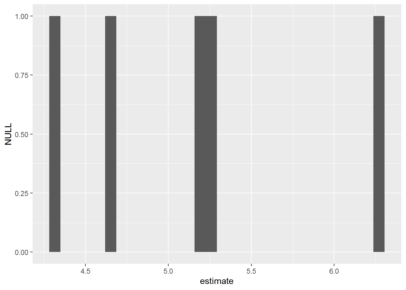
There are more variants of map() that you might find useful, both for simulations and in other iterative work. See the documentation for map() (?map) to see all of them along with additional examples.
Just the code, please
Here’s the code without all the discussion. Copy and paste the code below or you can download an R script of uncommented code from here.
library(purrr) # v. 0.2.5
suppressPackageStartupMessages( library(dplyr) ) # v. 0.7.5
library(ggplot2) # v 2.2.1

set.seed(16)
rnorm(5, mean = 0, sd = 1)

set.seed(16)
replicate(n = 3, rnorm(5, 0, 1), simplify = FALSE )

set.seed(16)
replicate(n = 3, rnorm(5, 0, 1) )

set.seed(16)
list1 = list() # Make an empty list to save output in
for (i in 1:3) { # Indicate number of iterations with "i"
    list1[[i]] = rnorm(5, 0, 1) # Save output in list for each iteration
}
list1

twogroup_fun = function(nrep = 10, b0 = 5, b1 = -2, sigma = 2) {
     ngroup = 2
     group = rep( c("group1", "group2"), each = nrep)
     eps = rnorm(ngroup*nrep, 0, sigma)
     growth = b0 + b1*(group == "group2") + eps
     growthfit = lm(growth ~ group)
     growthfit
}
twogroup_fun()

sim_lm = replicate(5, twogroup_fun(), simplify = FALSE )
length(sim_lm)

map(sim_lm, coef)

map_dbl(sim_lm, ~summary(.x)$r.squared)

map_dbl(sim_lm, function(x) summary(x)$r.squared)

map_dfr(sim_lm, broom::tidy)

map_dfr(sim_lm, broom::tidy, .id = "model")

map_dfr(sim_lm, broom::tidy, conf.int = TRUE)

sim_lm %>%
     map_dfr(broom::tidy) %>%
     filter(term == "(Intercept)") %>%
     qplot(x = estimate, data = ., geom = "histogram")