The small multiples plot: how to combine ggplot2 plots with one shared axis
There are a variety of ways to combine ggplot2 plots with a single shared axis. However, things can get tricky if you want a lot of control over all plot elements.
I demonstrate four different approaches for this:
1. Using facets, which is built in to ggplot2 but doesn’t allow much control over the non-shared axes.
2. Using package cowplot, which has a lot of nice features but the plot spacing doesn’t play well with a single shared axis.
3. Using package egg.
4. Using package patchwork.
The last two packages allow nice spacing for plots with a shared axis.
Table of Contents
Load R packages
I’ll be plotting with ggplot2, reshaping with tidyr, and combining plots with packages egg and patchwork.
I’ll also be using package cowplot version 0.9.4 to combine individual plots into one, but will use the package functions via cowplot:: instead of loading the package. (I believe the next version of cowplot will not be so opinionated about the theme.)
library(ggplot2) # v. 3.1.1
library(tidyr) # v. 0.8.3
library(egg) # v. 0.4.2
library(patchwork) # v. 1.0.0
The set-up
Here’s the scenario: we have one response variable (resp) that we want to plot against three other variables and combine them into a single “small multiples” plot.
I’ll call the three variables elev, grad, and slp. You’ll note that I created these variables to have very different scales.
set.seed(16)
dat = data.frame(elev = round( runif(20, 100, 500), 1),
                 resp = round( runif(20, 0, 10), 1),
                 grad = round( runif(20, 0, 1), 2),
                 slp = round( runif(20, 0, 35),1) )
head(dat)
# elev resp grad slp
# 1 373.2 9.7 0.05 8.8
# 2 197.6 8.1 0.42 33.3
# 3 280.0 5.4 0.38 19.3
# 4 191.8 4.3 0.07 29.6
# 5 445.4 2.3 0.43 16.5
# 6 224.5 6.5 0.78 4.1Using facets for small multiples
One good option when we want to make a similar plot for different groups (in this case, different variables) is to use faceting to make different panels within the same plot.
Since the three variables are currently in separate columns we’ll need to reshape the dataset prior to plotting. I’ll use gather() from tidyr for this.
datlong = gather(dat, key = "variable", value = "value", -resp)
head(datlong)
# resp variable value
# 1 9.7 elev 373.2
# 2 8.1 elev 197.6
# 3 5.4 elev 280.0
# 4 4.3 elev 191.8
# 5 2.3 elev 445.4
# 6 6.5 elev 224.5Now I can use facet_wrap() to make a separate scatterplot of resp vs each variable. The argument scales = "free_x" allows the x axis scales to differ for each variable but leaves a single y axis.
ggplot(datlong, aes(x = value, y = resp) ) +
     geom_point() +
     theme_bw() +
     facet_wrap(~variable, scales = "free_x")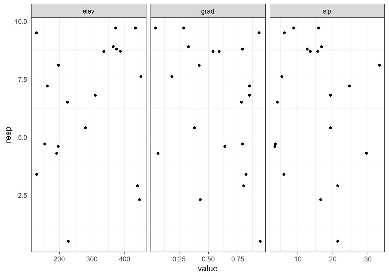
I can use the facet strips to give the appearance of axis labels, as shown in this Stack Overflow answer.
ggplot(datlong, aes(x = value, y = resp) ) +
     geom_point() +
     theme_bw() +
     facet_wrap(~variable, scales = "free_x", strip.position = "bottom") +
     theme(strip.background = element_blank(),
           strip.placement = "outside") +
     labs(x = NULL)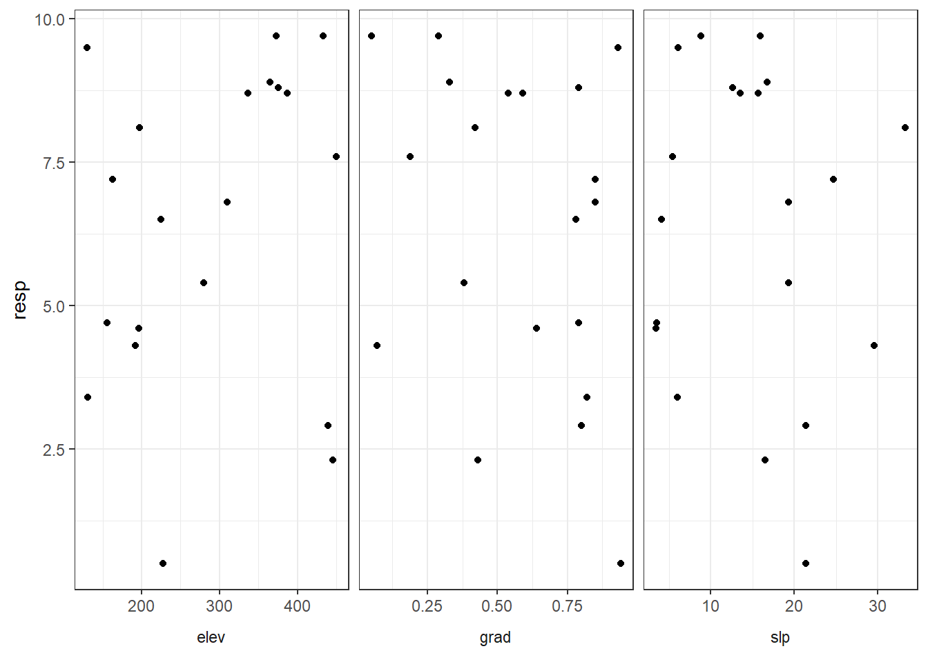
That’s a pretty nice plot to start with. However, controlling the axis breaks in the individual panels can be complicated, which is something we’d commonly want to do.
In that case, it may make more sense to create separate plots and then combine them into a small multiples plot with an add-on package.
Using cowplot to combine plots
Package cowplot is a really nice package for combining plots, and has lots of bells and whistles along with some pretty thorough vignettes.
The first step is to make each of the three plots separately. If doing lots of these we’d want to use some sort of loop to make a list of plots as I’ve demonstrated previously. Today I’m going to make the three plots manually.
elevplot = ggplot(dat, aes(x = elev, y = resp) ) +
     geom_point() +
     theme_bw()

gradplot = ggplot(dat, aes(x = grad, y = resp) ) +
     geom_point() +
     theme_bw() +
     scale_x_continuous(breaks = seq(0, 1, by = 0.2) )

slpplot = ggplot(dat, aes(x = slp, y = resp) ) +
     geom_point() +
     theme_bw() +
     scale_x_continuous(breaks = seq(0, 35, by = 5) )
The function plot_grid() in cowplot is for combining plots. To make a single row of plots I use nrow = 1.
The labels argument puts separate labels on each panel for captioning.
cowplot::plot_grid(elevplot,
                   gradplot,
                   slpplot,
                   nrow = 1,
                   labels = "auto")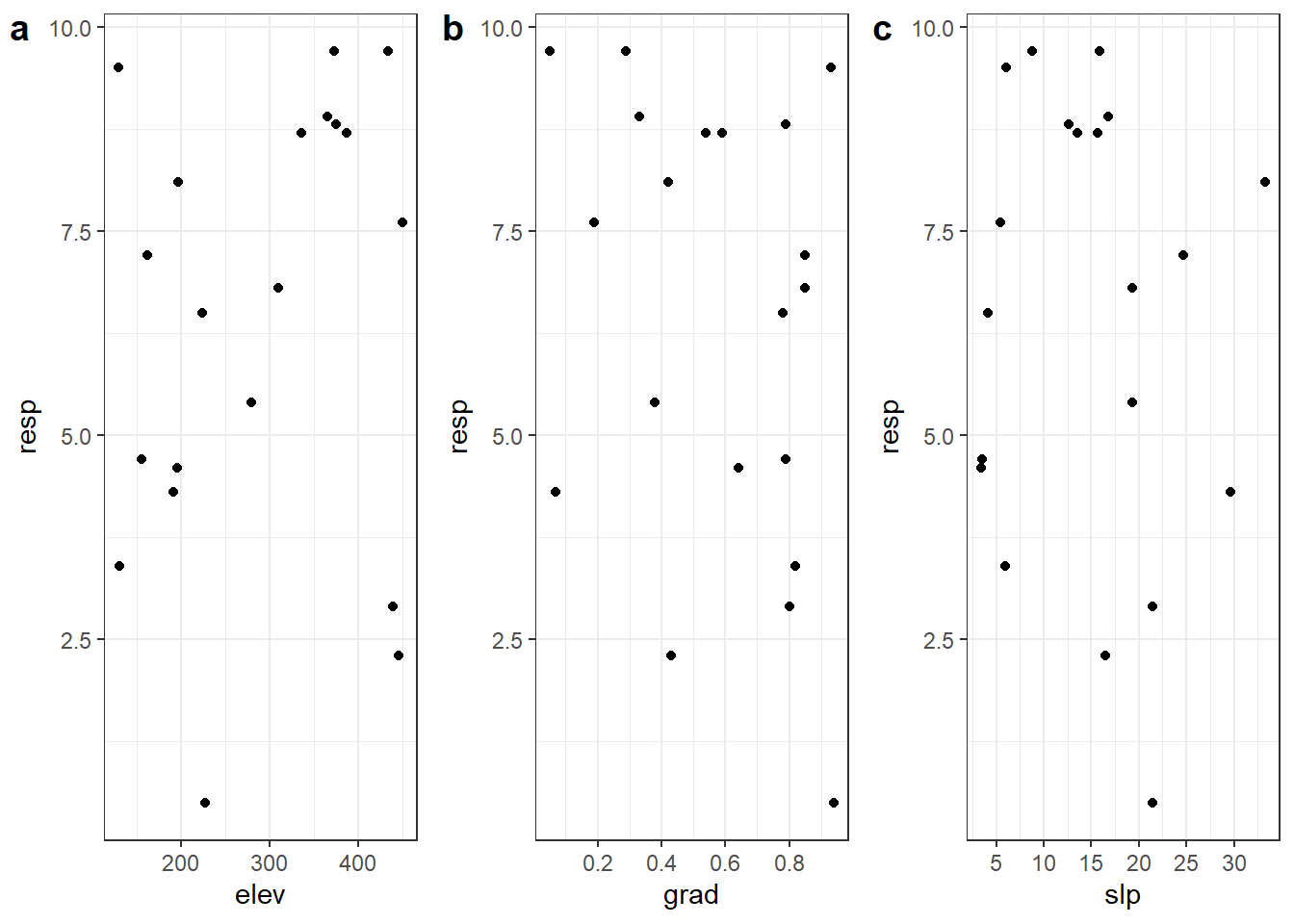
But we want a single shared y axis, not a separate y axis on each plot. I’ll remake the combined plot, this time removing the y axis elements from all but the first plot.
cowplot::plot_grid(elevplot,
                   gradplot + theme(axis.text.y = element_blank(),
                                    axis.ticks.y = element_blank(),
                                    axis.title.y = element_blank() ),
                   slpplot + theme(axis.text.y = element_blank(),
                                    axis.ticks.y = element_blank(),
                                    axis.title.y = element_blank() ),
                   nrow = 1,
                   labels = "auto")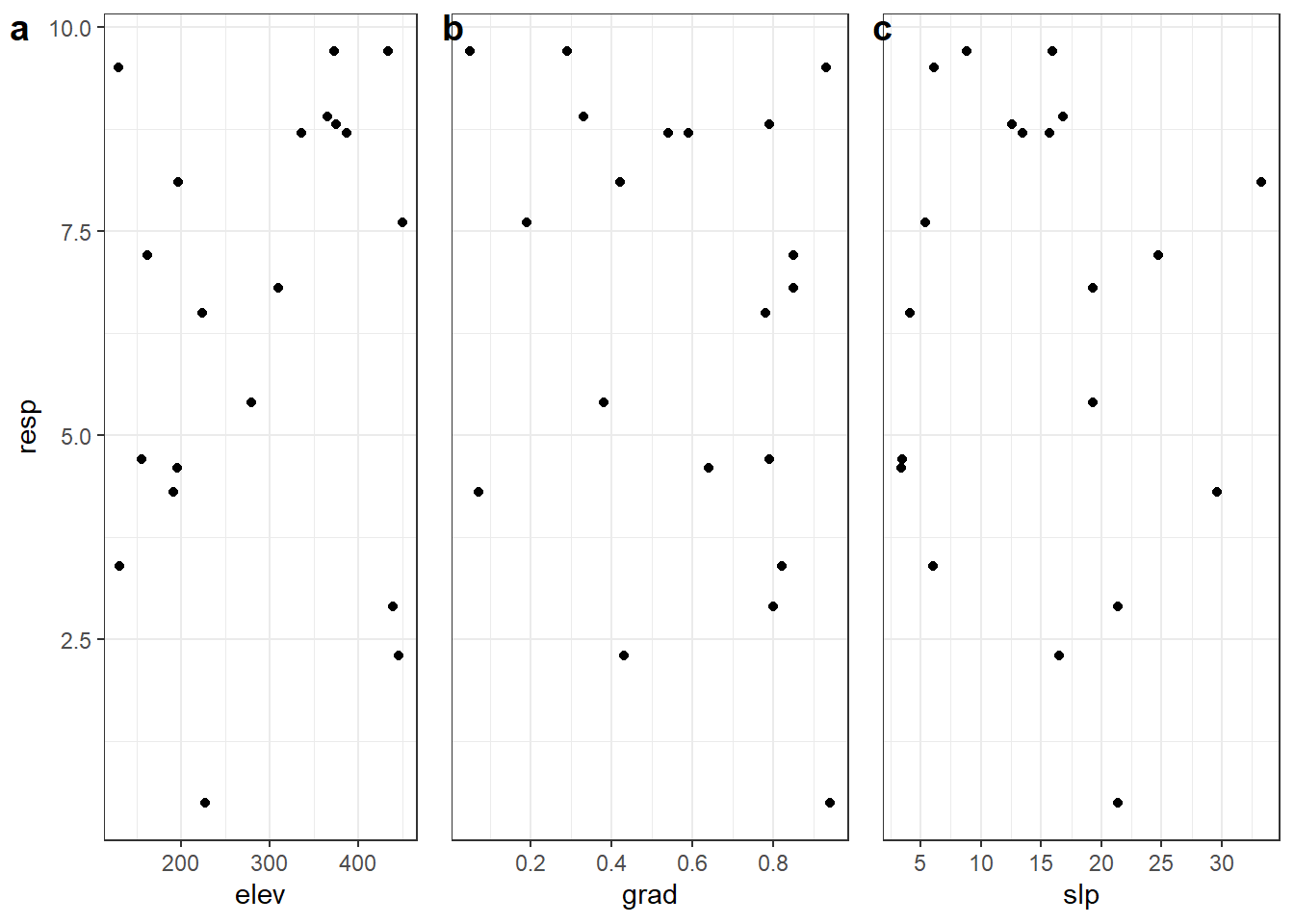
This makes panels different sizes, though, which isn’t ideal. To have all the plots the same width I need to align them vertically with align = "v".
cowplot::plot_grid(elevplot,
                   gradplot +
                        theme(axis.text.y = element_blank(),
                              axis.ticks.y = element_blank(),
                              axis.title.y = element_blank() ),
                   slpplot +
                        theme(axis.text.y = element_blank(),
                              axis.ticks.y = element_blank(),
                              axis.title.y = element_blank() ),
                   nrow = 1,
                   labels = "auto",
                   align = "v")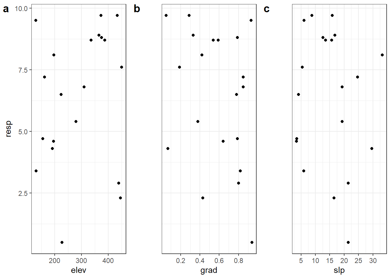
But, unfortunately, this puts the axis space back between the plots to make them all the same width. It turns out that cowplot isn’t really made for plots with a single shared axis. The cowplot package author points us to package egg for this in this Stack Overflow answer.
Using egg to combine plots
Package egg is another nice alternative for combining plots into a small multiples plot. The function in this package for combining plots is called ggarrange().
Here are the three plots again.
elevplot = ggplot(dat, aes(x = elev, y = resp) ) +
     geom_point() +
     theme_bw()

gradplot = ggplot(dat, aes(x = grad, y = resp) ) +
     geom_point() +
     theme_bw() +
     scale_x_continuous(breaks = seq(0, 1, by = 0.2) )

slpplot = ggplot(dat, aes(x = slp, y = resp) ) +
     geom_point() +
     theme_bw() +
     scale_x_continuous(breaks = seq(0, 35, by = 5) )
The ggarrange() function has an nrow argument so I can keep the plots in a single row.
The panel spacing is automagically the same here after I remove the y axis elements, and things look pretty nice right out of the box.
ggarrange(elevplot,
          gradplot +
               theme(axis.text.y = element_blank(),
                     axis.ticks.y = element_blank(),
                     axis.title.y = element_blank() ),
          slpplot +
               theme(axis.text.y = element_blank(),
                     axis.ticks.y = element_blank(),
                     axis.title.y = element_blank() ),
          nrow = 1)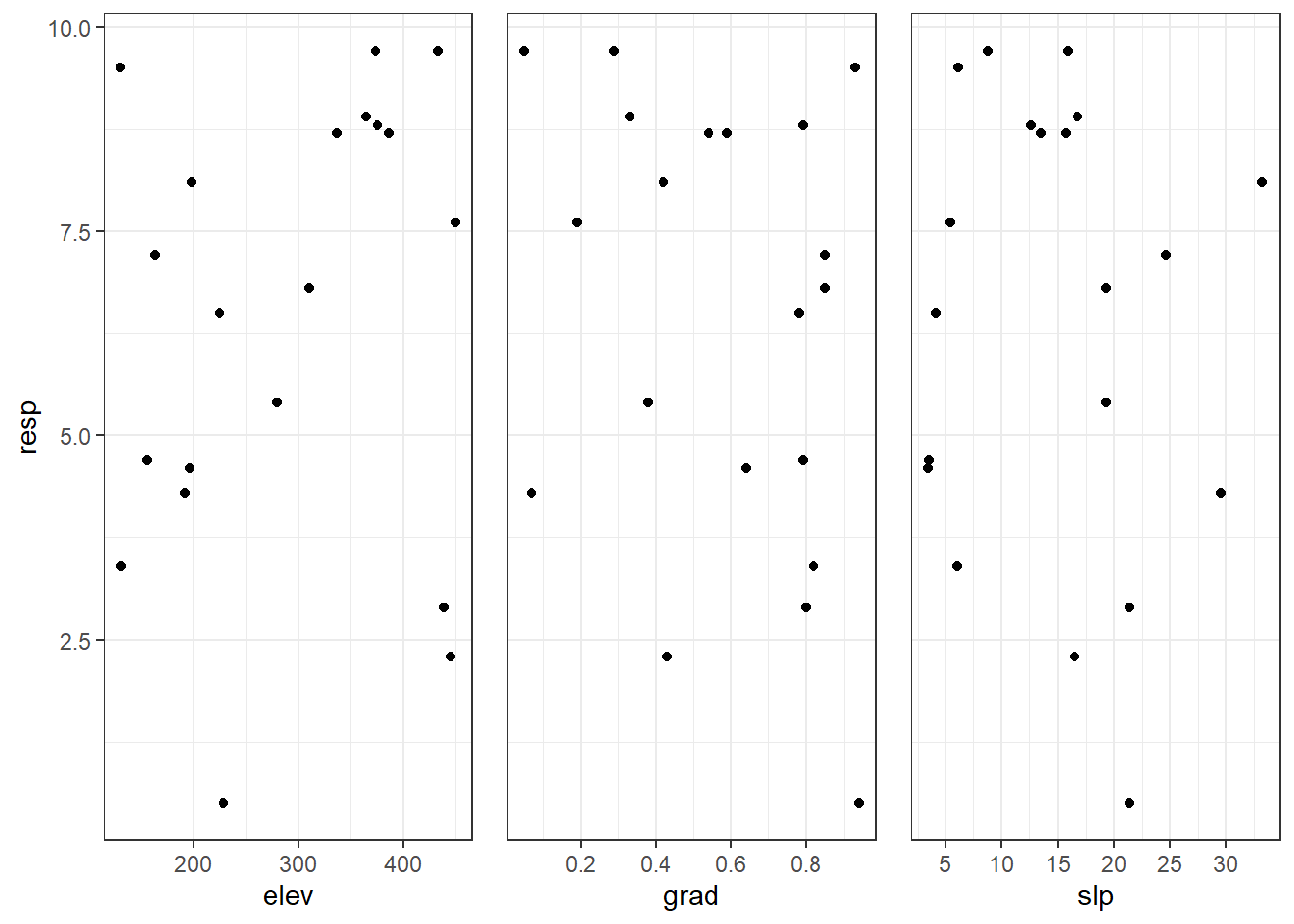
We can bring panes closer by removing some of the space around the plot margins with the plot.margin in theme(). I’ll set the spacing for right margin of the first plot, both left and right margins of the second, and the left margin of the third.
ggarrange(elevplot +
               theme(axis.ticks.y = element_blank(),
                     plot.margin = margin(r = 1) ),
          gradplot +
               theme(axis.text.y = element_blank(),
                     axis.ticks.y = element_blank(),
                     axis.title.y = element_blank(),
                     plot.margin = margin(r = 1, l = 1) ),
          slpplot +
               theme(axis.text.y = element_blank(),
                     axis.ticks.y = element_blank(),
                     axis.title.y = element_blank(),
                     plot.margin = margin(l = 1)  ),
          nrow = 1)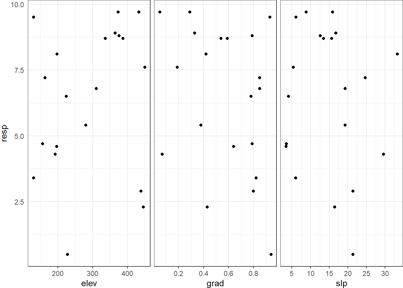
Adding plot labels with tag_facet()
You’ll see there is a labels argument in ggarrange() documentation, but it didn’t work well for me out of the box with only one plot with a y axis. However, we can get tricky with egg::tag_facet() if we add a facet strip to each of the individual plots.
It’d make sense to build these plots outside of ggarrange() and then add the tags and combine them instead of nesting everything like I did here, since the code is now a little hard to follow.
ggarrange(tag_facet(elevplot +
                          theme(axis.ticks.y = element_blank(),
                                plot.margin = margin(r = 1) ) +
                          facet_wrap(~"elev"),
                     tag_pool = "a"),
          tag_facet(gradplot +
                          theme(axis.text.y = element_blank(),
                                axis.ticks.y = element_blank(),
                                axis.title.y = element_blank(),
                                plot.margin = margin(r = 1, l = 1) ) +
                          facet_wrap(~"grad"),
                    tag_pool = "b" ),
          tag_facet(slpplot +
                          theme(axis.text.y = element_blank(),
                                axis.ticks.y = element_blank(),
                                axis.title.y = element_blank(),
                                plot.margin = margin(l = 1)  ) +
                          facet_wrap(~"slp"),
                     tag_pool = "c"),
          nrow = 1)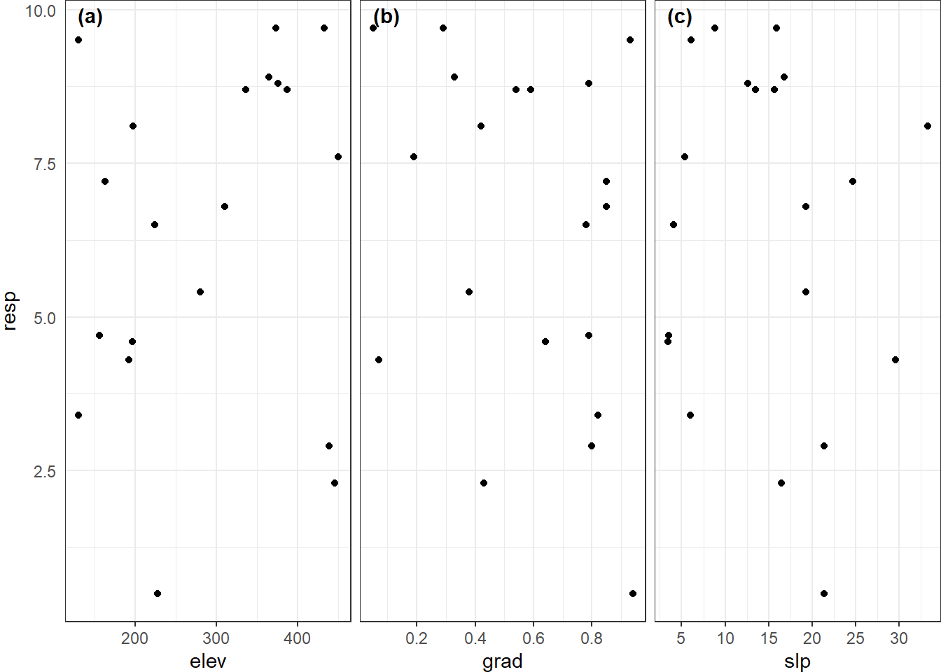
We might want to add a right y axis to the right-most plot. In this case we’d want to change the axis ticks length to 0 via theme() elements. This can be done separately per axis in the development version of ggplot2, and will be included in version 3.2.0.
Using patchwork to combine plots
The patchwork package is another one that is great for combining plots, and is now on CRAN (as of December 2019) 🎉. It has nice vignettes here to help you get started.
In patchwork the + operator is used to add plots together. Here’s an example, combining my three original plots.
elevplot + gradplot + slpplot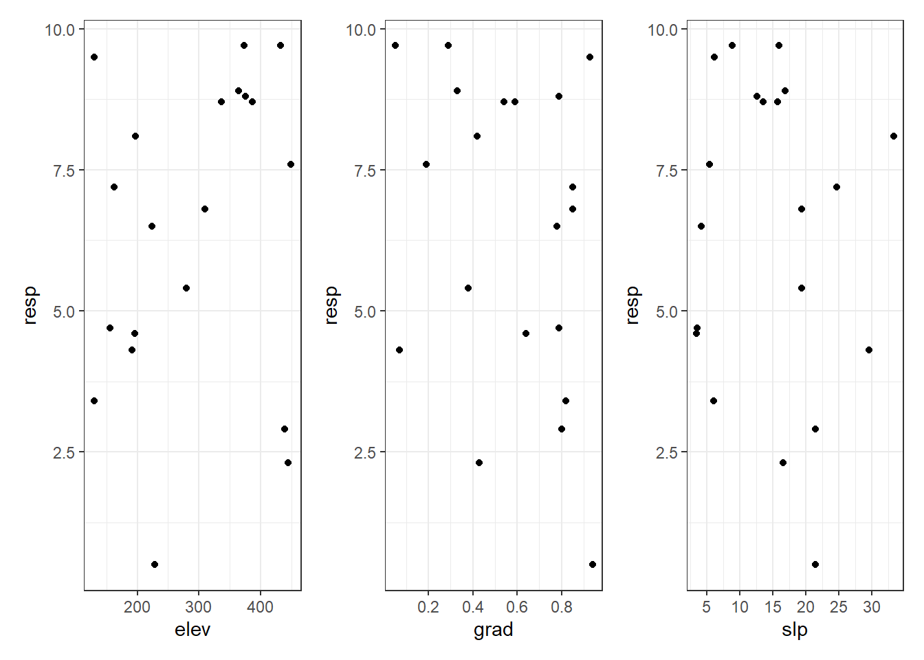
If we give the resulting combined plot a name, we can remove the titles from the last two subplots using double-bracket indexing. (Of course, I also could have built the plots how I wanted them in the first place. 😜)
The result has nice spacing for a single, shared y axis. Margins can be controlled the same was as in the egg example above.
patchwork = elevplot + gradplot + slpplot

# Remove title from second subplot
patchwork[[2]] = patchwork[[2]] + theme(axis.text.y = element_blank(),
                                        axis.ticks.y = element_blank(),
                                        axis.title.y = element_blank() )

# Remove title from third subplot
patchwork[[3]] = patchwork[[3]] + theme(axis.text.y = element_blank(),
                                        axis.ticks.y = element_blank(),
                                        axis.title.y = element_blank() )

patchwork
Adding plots labels with plot_annotation()
There are many annotation options in patchwork. I’ll focus on adding tags, but see the annotation vignette.
Tags can be added with the tag_levels argument in plot_annotation(). I want lowercase Latin letter so use "a" as my tag_levels.
Plot tags go outside the plot by default. You can control the position at least somewhat with the theme option plot.tag.position, which works on the individual subplots and not the entire combined plot.
patchwork + plot_annotation(tag_levels = "a")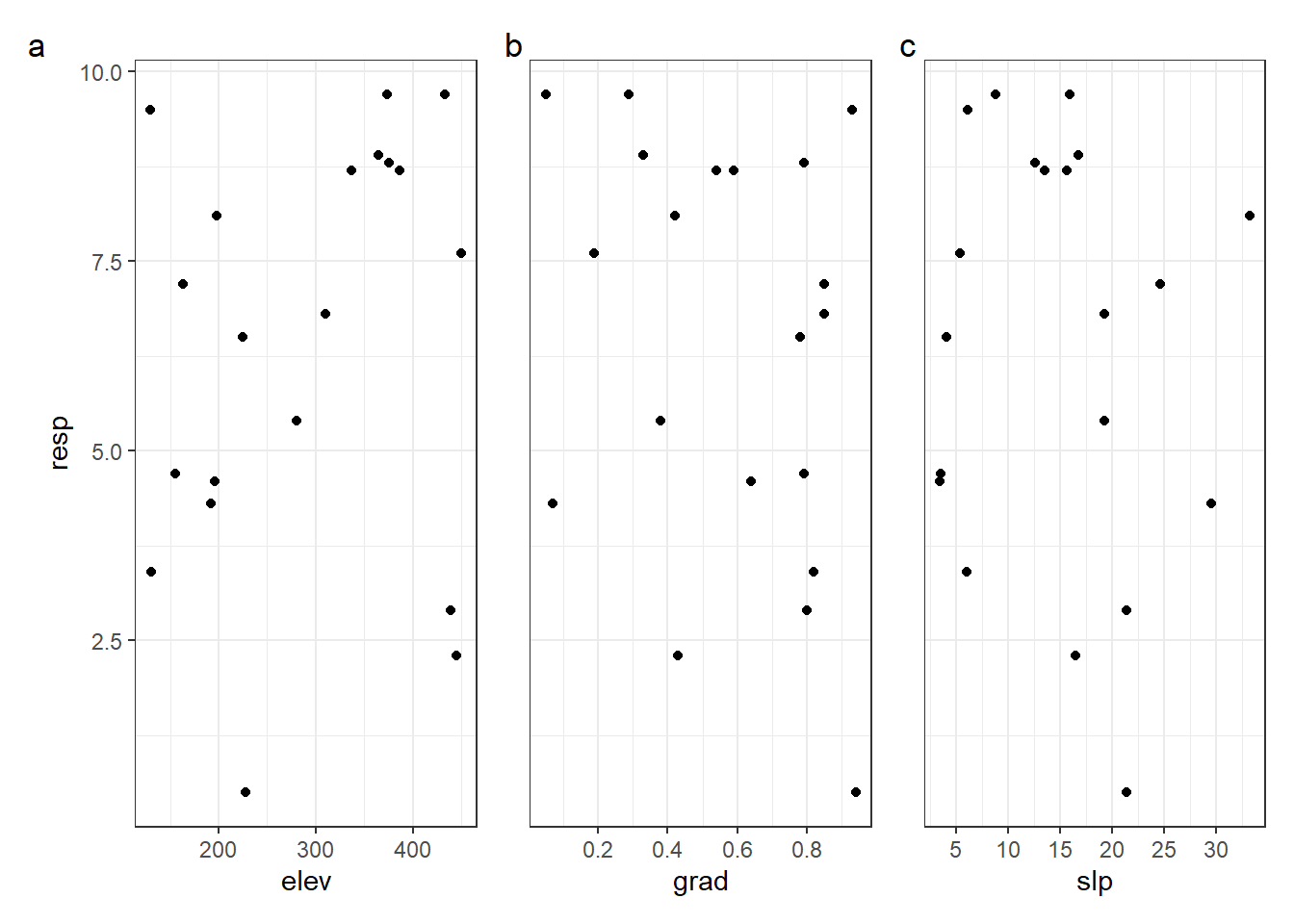
Just the code, please
Here’s the code without all the discussion. Copy and paste the code below or you can download an R script of uncommented code from here.
library(ggplot2) # v. 3.1.1
library(tidyr) # v. 0.8.3
library(egg) # v. 0.4.2
library(patchwork) # v. 1.0.0

set.seed(16)
dat = data.frame(elev = round( runif(20, 100, 500), 1),
                 resp = round( runif(20, 0, 10), 1),
                 grad = round( runif(20, 0, 1), 2),
                 slp = round( runif(20, 0, 35),1) )
head(dat)

datlong = gather(dat, key = "variable", value = "value", -resp)
head(datlong)

ggplot(datlong, aes(x = value, y = resp) ) +
     geom_point() +
     theme_bw() +
     facet_wrap(~variable, scales = "free_x")

ggplot(datlong, aes(x = value, y = resp) ) +
     geom_point() +
     theme_bw() +
     facet_wrap(~variable, scales = "free_x", strip.position = "bottom") +
     theme(strip.background = element_blank(),
           strip.placement = "outside") +
     labs(x = NULL)

elevplot = ggplot(dat, aes(x = elev, y = resp) ) +
     geom_point() +
     theme_bw()

gradplot = ggplot(dat, aes(x = grad, y = resp) ) +
     geom_point() +
     theme_bw() +
     scale_x_continuous(breaks = seq(0, 1, by = 0.2) )

slpplot = ggplot(dat, aes(x = slp, y = resp) ) +
     geom_point() +
     theme_bw() +
     scale_x_continuous(breaks = seq(0, 35, by = 5) )

cowplot::plot_grid(elevplot,
                   gradplot,
                   slpplot,
                   nrow = 1,
                   labels = "auto")

cowplot::plot_grid(elevplot,
                   gradplot + theme(axis.text.y = element_blank(),
                                    axis.ticks.y = element_blank(),
                                    axis.title.y = element_blank() ),
                   slpplot + theme(axis.text.y = element_blank(),
                                    axis.ticks.y = element_blank(),
                                    axis.title.y = element_blank() ),
                   nrow = 1,
                   labels = "auto")

cowplot::plot_grid(elevplot,
                   gradplot +
                        theme(axis.text.y = element_blank(),
                              axis.ticks.y = element_blank(),
                              axis.title.y = element_blank() ),
                   slpplot +
                        theme(axis.text.y = element_blank(),
                              axis.ticks.y = element_blank(),
                              axis.title.y = element_blank() ),
                   nrow = 1,
                   labels = "auto",
                   align = "v")

elevplot = ggplot(dat, aes(x = elev, y = resp) ) +
     geom_point() +
     theme_bw()

gradplot = ggplot(dat, aes(x = grad, y = resp) ) +
     geom_point() +
     theme_bw() +
     scale_x_continuous(breaks = seq(0, 1, by = 0.2) )

slpplot = ggplot(dat, aes(x = slp, y = resp) ) +
     geom_point() +
     theme_bw() +
     scale_x_continuous(breaks = seq(0, 35, by = 5) )

ggarrange(elevplot,
          gradplot +
               theme(axis.text.y = element_blank(),
                     axis.ticks.y = element_blank(),
                     axis.title.y = element_blank() ),
          slpplot +
               theme(axis.text.y = element_blank(),
                     axis.ticks.y = element_blank(),
                     axis.title.y = element_blank() ),
          nrow = 1)

ggarrange(elevplot +
               theme(axis.ticks.y = element_blank(),
                     plot.margin = margin(r = 1) ),
          gradplot +
               theme(axis.text.y = element_blank(),
                     axis.ticks.y = element_blank(),
                     axis.title.y = element_blank(),
                     plot.margin = margin(r = 1, l = 1) ),
          slpplot +
               theme(axis.text.y = element_blank(),
                     axis.ticks.y = element_blank(),
                     axis.title.y = element_blank(),
                     plot.margin = margin(l = 1)  ),
          nrow = 1)

ggarrange(tag_facet(elevplot +
                          theme(axis.ticks.y = element_blank(),
                                plot.margin = margin(r = 1) ) +
                          facet_wrap(~"elev"),
                     tag_pool = "a"),
          tag_facet(gradplot +
                          theme(axis.text.y = element_blank(),
                                axis.ticks.y = element_blank(),
                                axis.title.y = element_blank(),
                                plot.margin = margin(r = 1, l = 1) ) +
                          facet_wrap(~"grad"),
                    tag_pool = "b" ),
          tag_facet(slpplot +
                          theme(axis.text.y = element_blank(),
                                axis.ticks.y = element_blank(),
                                axis.title.y = element_blank(),
                                plot.margin = margin(l = 1)  ) +
                          facet_wrap(~"slp"),
                     tag_pool = "c"),
          nrow = 1)

elevplot + gradplot + slpplot

patchwork = elevplot + gradplot + slpplot

# Remove title from second subplot
patchwork[[2]] = patchwork[[2]] + theme(axis.text.y = element_blank(),
                                        axis.ticks.y = element_blank(),
                                        axis.title.y = element_blank() )

# Remove title from third subplot
patchwork[[3]] = patchwork[[3]] + theme(axis.text.y = element_blank(),
                                        axis.ticks.y = element_blank(),
                                        axis.title.y = element_blank() )

patchwork

patchwork + plot_annotation(tag_levels = "a")