Many similar models - Part 1: How to make a function for model fitting
This post was last updated on 2022-01-05.
I worked with several students over the last few months who were fitting many linear models, all with the same basic structure but different response variables. They were struggling to find an efficient way to do this in R while still taking the time to check model assumptions.
A first step when working towards a more automated process for fitting many models is to learn how to build model formulas using reformulate() or with paste() and as.formula(). Once we learn how to build model formulas we can create functions to streamline the model fitting process.
I will be making residuals plots with ggplot2 today so will load it here.
library(ggplot2) # v.3.2.0Table of Contents
- Building a formula with reformulate()
- Using a constructed formula in lm()
- Making a function for model fitting
- Using bare names instead of strings (i.e., non-standard evaluation)
- Building a formula with varying explanatory variables
- The dots for passing many variables to a function
- Example function that returns residuals plots and model output
- Next step: looping
- Just the code, please
Building a formula with reformulate()
Model formula of the form y ~ x can be built based on variable names passed as character strings. A character string means the variable name will have quotes around it.
The function reformulate() allows us to pass response and explanatory variables as character strings and returns them as a formula.
Here is an example, using mpg as the response variable and am as the explanatory variable. Note the explanatory variable is passed to the first argument, termlabels, and the response variable to response.
reformulate(termlabels = "am", response = "mpg")# mpg ~ amA common alternative to reformulate() is to use paste() with as.formula(). I show this option below, but won’t discuss it more in this post.
as.formula( paste("mpg", "~ am") )# mpg ~ amUsing a constructed formula in lm()
Once we’ve built the formula we can put it in as the first argument of a model fitting function like lm() in order to fit the model. I’ll be using the mtcars dataset throughout the model fitting examples.
Since am is a 0/1 variable, this particular analysis is a two-sample t-test with mpg as the response variable. I removed the step of writing out the first argument name to reformulate to save space, knowing that the first argument is always the explanatory variables.
lm( reformulate("am", response = "mpg"), data = mtcars)#
# Call:
# lm(formula = reformulate("am", response = "mpg"), data = mtcars)
#
# Coefficients:
# (Intercept) am
# 17.147 7.245Making a function for model fitting
Being able to build a formula is essential for making user-defined model fitting functions.
For example, say I wanted to do the same t-test with am for many response variables. I could create a function that takes the response variable as an argument and build the model formula within the function with reformulate().
The response variable name is passed to the response argument as a character string.
lm_fun = function(response) {
  lm( reformulate("am", response = response), data = mtcars)
}
Here are two examples of this function in action, using mpg and then wt as the response variables.
lm_fun(response = "mpg")#
# Call:
# lm(formula = reformulate("am", response = response), data = mtcars)
#
# Coefficients:
# (Intercept) am
# 17.147 7.245lm_fun(response = "wt")#
# Call:
# lm(formula = reformulate("am", response = response), data = mtcars)
#
# Coefficients:
# (Intercept) am
# 3.769 -1.358Using bare names instead of strings (i.e., non-standard evaluation)
As you can see, this approach to building formula relies on character strings. This is going to be great once we start looping through variable names, but if making a function for interactive use it can be nice for the user to pass bare column names.
We can use some deparse()/substitute() magic in the function for this. Those two functions will turn bare names into strings within the function rather than having the user pass strings directly.
lm_fun2 = function(response) {
  resp = deparse( substitute( response) )
  lm( reformulate("am", response = resp), data = mtcars)
}
Here’s an example of this function in action. Note the use of the bare column name for the response variable.
lm_fun2(response = mpg)#
# Call:
# lm(formula = reformulate("am", response = resp), data = mtcars)
#
# Coefficients:
# (Intercept) am
# 17.147 7.245You can see that one thing that happens when using reformulate() like this is that the formula in the model output shows the formula-building code instead of the actual variables used in the model.
Call:
lm(formula = reformulate("am", response = resp), data = mtcars)
While this often won’t matter in practice, there are ways to force the model to show the variables used in the model fitting. See this blog post for some discussion as well as code for how to do this.
Building a formula with varying explanatory variables
The formula building approach can also be used for fitting models where the explanatory variables vary. The explanatory variables should have plus signs between them on the right-hand side of the formula, which we can achieve by passing a vector of character strings to the first argument of reformulate().
expl = c("am", "disp")
reformulate(expl, response = "mpg")
# mpg ~ am + dispLet’s go through an example of using this in a function that can fit a model with different explanatory variables.
In this function I demonstrate building the formula as a separate step and then passing it to lm(). Some find this easier to read compared to building the formula within lm() as a single step like I did earlier.
lm_fun_expl = function(expl) {
  form = reformulate(expl, response = "mpg")
  lm(form, data = mtcars)
}
To use the function we pass a vector of variable names as strings to the expl argument.
lm_fun_expl(expl = c("am", "disp") )#
# Call:
# lm(formula = form, data = mtcars)
#
# Coefficients:
# (Intercept) am disp
# 27.84808 1.83346 -0.03685The dots for passing many variables to a function
Using dots (…) instead of named arguments can allow the user to list the explanatory variables separately instead of in a vector.
I’ll demonstrate a function using dots to indicate some undefined number of additional arguments for putting as many explanatory variables as desired into the model. I wrap the dots in c() within the function in order to collapse variables together with +.
lm_fun_expl2 = function(...) {
  form = reformulate(c(...), response = "mpg")
  lm(form, data = mtcars)
}
Now variables are passed individually as strings separated by commas instead of as a vector.
lm_fun_expl2("am", "disp")#
# Call:
# lm(formula = form, data = mtcars)
#
# Coefficients:
# (Intercept) am disp
# 27.84808 1.83346 -0.03685Example function that returns residuals plots and model output
One of the reasons to make a function is to increase efficiency when fitting many models. For example, it might be useful to make a function that returns residual plots and any desired statistical results simultaneously.
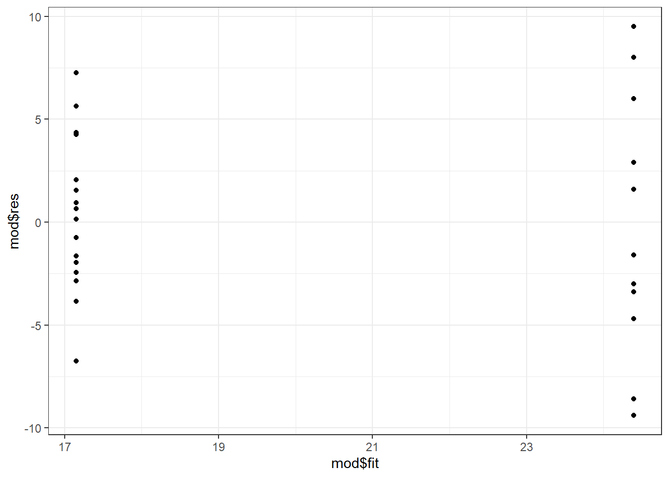
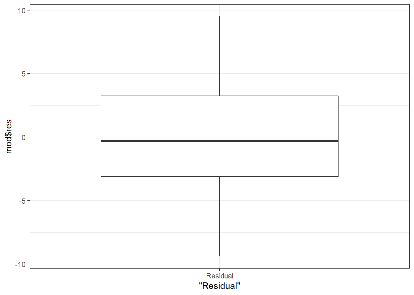
Here’s an example of such a function, using some of the tools covered above. The function takes the response variable as a bare name, fits a model with am hard-coded as the explanatory variable and the mtcars dataset, and then makes two residual plots.
The function outputs a list that contains the two residuals plots as well as the overall \(F\) tests from the model.
lm_modfit = function(response) {
  resp = deparse( substitute( response) )
  mod = lm( reformulate("am", response = resp), data = mtcars)
  resvfit = qplot(x = mod$fit, y = mod$res) + theme_bw()
  resdist = qplot(x = "Residual", mod$res, geom = "boxplot") + theme_bw()
  list(resvfit, resdist, anova(mod) )
}

mpgfit = lm_modfit(mpg)
Individual parts of the output list can be extracted as needed. To check model assumptions prior to looking at any results we’d pull out the two plots, which are the first two elements of the output list.
mpgfit[1:2]# [[1]]
#
# [[2]]
If we deem the model fit acceptable we can extract the overall \(F\) tests from the third element of the output.
mpgfit[[3]]# Analysis of Variance Table
#
# Response: mpg
# Df Sum Sq Mean Sq F value Pr(>F)
# am 1 405.15 405.15 16.86 0.000285 ***
# Residuals 30 720.90 24.03
# ---
# Signif. codes: 0 '***' 0.001 '**' 0.01 '*' 0.05 '.' 0.1 ' ' 1Next step: looping
This post focused on using reformulate() for building model formula and then making user-defined functions for interactive use. When working with many models we’d likely want to automate the process more by using some sort of looping. I wrote a follow-up post on looping through variables and fitting models with the map family of functions from package purrr, which you can see here.
Just the code, please
Here’s the code without all the discussion. Copy and paste the code below or you can download an R script of uncommented code from here.
library(ggplot2) # v.3.2.0

reformulate(termlabels = "am", response = "mpg")

as.formula( paste("mpg", "~ am") )

lm( reformulate("am", response = "mpg"), data = mtcars)

lm_fun = function(response) {
  lm( reformulate("am", response = response), data = mtcars)
}

lm_fun(response = "mpg")
lm_fun(response = "wt")

lm_fun2 = function(response) {
  resp = deparse( substitute( response) )
  lm( reformulate("am", response = resp), data = mtcars)
}

lm_fun2(response = mpg)

expl = c("am", "disp")
reformulate(expl, response = "mpg")

lm_fun_expl = function(expl) {
  form = reformulate(expl, response = "mpg")
  lm(form, data = mtcars)
}

lm_fun_expl(expl = c("am", "disp") )

lm_fun_expl2 = function(...) {
  form = reformulate(c(...), response = "mpg")
  lm(form, data = mtcars)
}

lm_fun_expl2("am", "disp")

lm_modfit = function(response) {
  resp = deparse( substitute( response) )
  mod = lm( reformulate("am", response = resp), data = mtcars)
  resvfit = qplot(x = mod$fit, y = mod$res) + theme_bw()
  resdist = qplot(x = "Residual", mod$res, geom = "boxplot") + theme_bw()
  list(resvfit, resdist, anova(mod) )
}

mpgfit = lm_modfit(mpg)
mpgfit[1:2]
mpgfit[[3]]