Controlling legend appearance in ggplot2 with override.aes
In ggplot2, aesthetics and their scale_*() functions change both the plot appearance and the plot legend appearance simultaneously. The override.aes argument in guide_legend() allows the user to change only the legend appearance without affecting the rest of the plot. This is useful for making the legend more readable or for creating certain types of combined legends.
In this post I’ll first introduce override.aes with a basic example and then go through three additional plotting scenarios to how other instances where override.aes comes in handy.
Table of Contents
R packages
The only package I’ll use in this post is ggplot2 for plotting.
library(ggplot2) # v. 3.3.2Introducing override.aes
A basic reason to change the legend appearance without changing the plot is to make the legend more readable.
For example, I’ll start with a scatterplot using the diamonds dataset. This is a large dataset, so after mapping color to the cut variable I set alpha to increase the transparency and size to reduce the size of points in the plot.
You can see using alpha and size changes the way the points are shown in both the plot and the legend.
ggplot(data = diamonds, aes(x = carat, y = price, color = cut) ) +
     geom_point(alpha = .25, size = 1)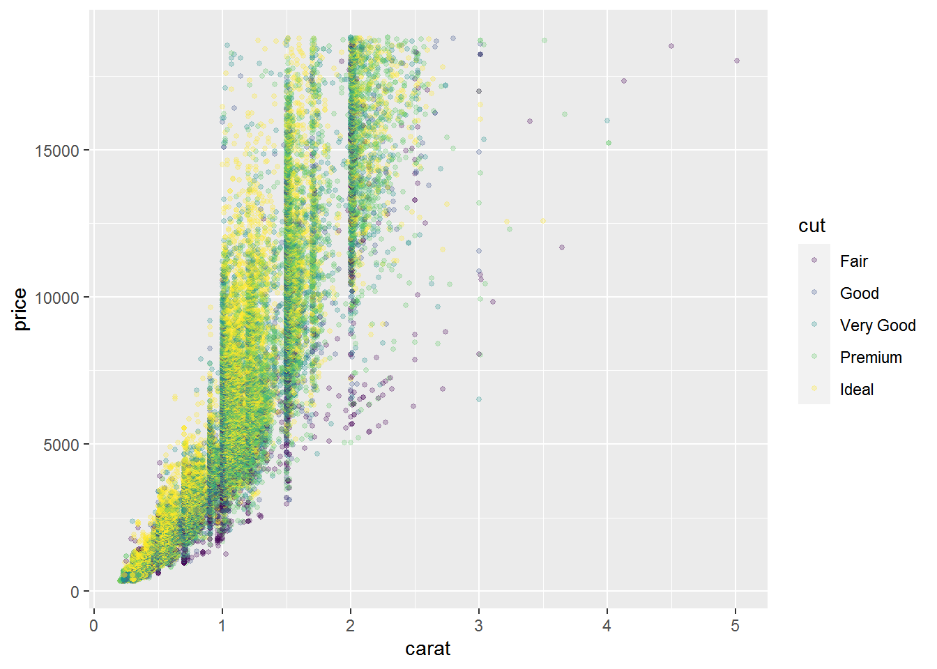
Adding a guides() layer
Making the points small and transparent may be desirable when plotting many points, but it also makes the legend more difficult to read. This is a case where I’d want to make the legend more readable by increasing the point size and/or reducing the point transparency.
One way to do this is by adding a guides() layer. The guides() function uses scale name-guide pairs. I am going to change the legend for the color scale, so I’ll use color = guide_legend() as the scale name-guide pair.
override.aes is an argument within guide_legend(), so if you’re looking for more background you can start at ?guide_legend. The override.aes argument takes a list of aesthetic parameters that will override the default legend appearance.
To increase the size of the points in the color legend of my plot, the layer I’ll add will look like:
guides(color = guide_legend(override.aes = list(size = 3) ) )Adding this layer to the initial plot, you can see how the points in the legend get larger while the points in the plot remain unchanged.
ggplot(data = diamonds, aes(x = carat, y = price, color = cut) ) +
     geom_point(alpha = .25, size = 1) +
     guides(color = guide_legend(override.aes = list(size = 3) ) )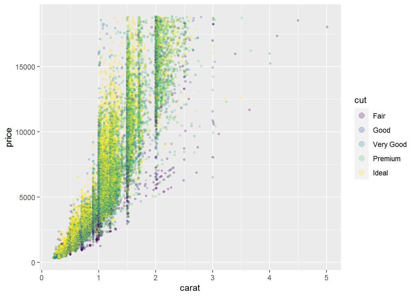
Using the guide argument in scale_*()
If I am going to change my default colors with a scale_color_*() function in addition to overriding the legend appearance, I can use the guide argument there instead of adding a separate guides() layer. The guide argument is part of all scale functions.
For example, say I am already using scale_color_viridis_d() to change the default color palette of the whole plot (i.e., plot and legend). I can use the same guide_legend() code from above for the guide argument to change the size of the points in the legend.
ggplot(data = diamonds, aes(x = carat, y = price, color = cut) ) +
     geom_point(alpha = .25, size = 1) +
     scale_color_viridis_d(option = "magma",
                           guide = guide_legend(override.aes = list(size = 3) ) )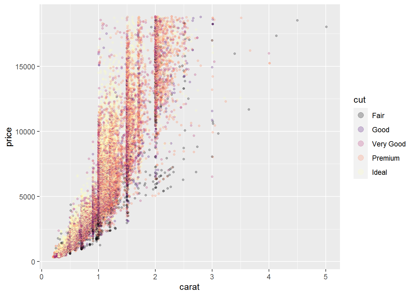
Changing multiple aesthetic parameters
You can control multiple aesthetic parameters at once by adding them to the list passed to override.aes. If I want to increase the point size as well as remove the point transparency in the legend, I can change both size and alpha.
ggplot(data = diamonds, aes(x = carat, y = price, color = cut) ) +
     geom_point(alpha = .25, size = 1) +
     scale_color_viridis_d(option = "magma",
                           guide = guide_legend(override.aes = list(size = 3,
                                                                    alpha = 1) ) )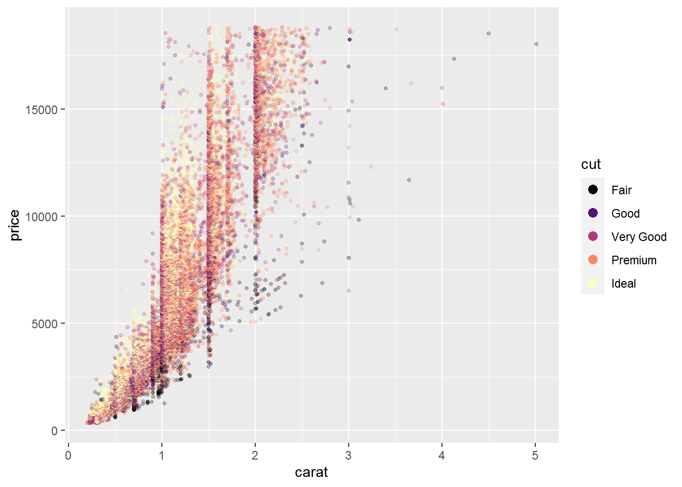
Suppress aesthetics from part of the legend
Removing aesthetic for only some parts of the legend is another use for override.aes. For example, this can be useful when different layers are based on a different number of levels for the same grouping factor.
The following example is based on this Stack Overflow question. The points data has information from all three groups of the id variable but the rectangle, based on the box dataset, is for only a single group.
points = structure(list(x = c(5L, 10L, 7L, 9L, 86L, 46L, 22L, 94L, 21L,
6L, 24L, 3L), y = c(51L, 54L, 50L, 60L, 97L, 74L, 59L, 68L, 45L,
56L, 25L, 70L), id = c("a", "a", "a", "a", "b", "b", "b", "b",
"c", "c", "c", "c")), row.names = c(NA, -12L), class = "data.frame")

head(points)
# x y id
# 1 5 51 a
# 2 10 54 a
# 3 7 50 a
# 4 9 60 a
# 5 86 97 b
# 6 46 74 bbox = data.frame(left = 1, right = 10, bottom = 50, top = 60, id = "a")
box# left right bottom top id
# 1 1 10 50 60 aHere’s what the initial plot looks like, mapping color to the id variable. Note that the colored outlines, representing the rectangle layer, are present for every group in the legend even though there is a rectangle for only one of the groups present in the plot.
ggplot(data = points, aes(color = id) ) +
geom_point(aes(x = x, y = y), size = 4) +
geom_rect(data = box, aes(xmin = left,
xmax = right,
ymin = 50,
ymax = top),
fill = NA, size = 1)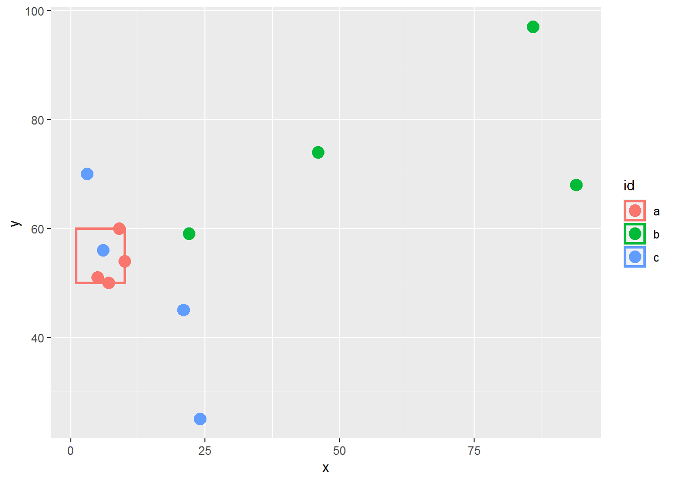
In this case, I want to remove the outlines for the second and third legend key boxes so the legend matches what is in the plot. The legend outlines are based on the linetype aesthetic. Suppressing these lines can be done with override.aes, setting the line types to 0 in order to remove them.
Note that I have to list the line type for every group, not just the groups I want to remove. I keep the line for the first group solid via 1.
ggplot(data = points, aes(color = id) ) +
geom_point(aes(x = x, y = y), size = 4) +
geom_rect(data = box, aes(xmin = left,
xmax = right,
ymin = 50,
ymax = top),
fill = NA, size = 1) +
guides(color = guide_legend(override.aes = list(linetype = c(1, 0, 0) ) ) )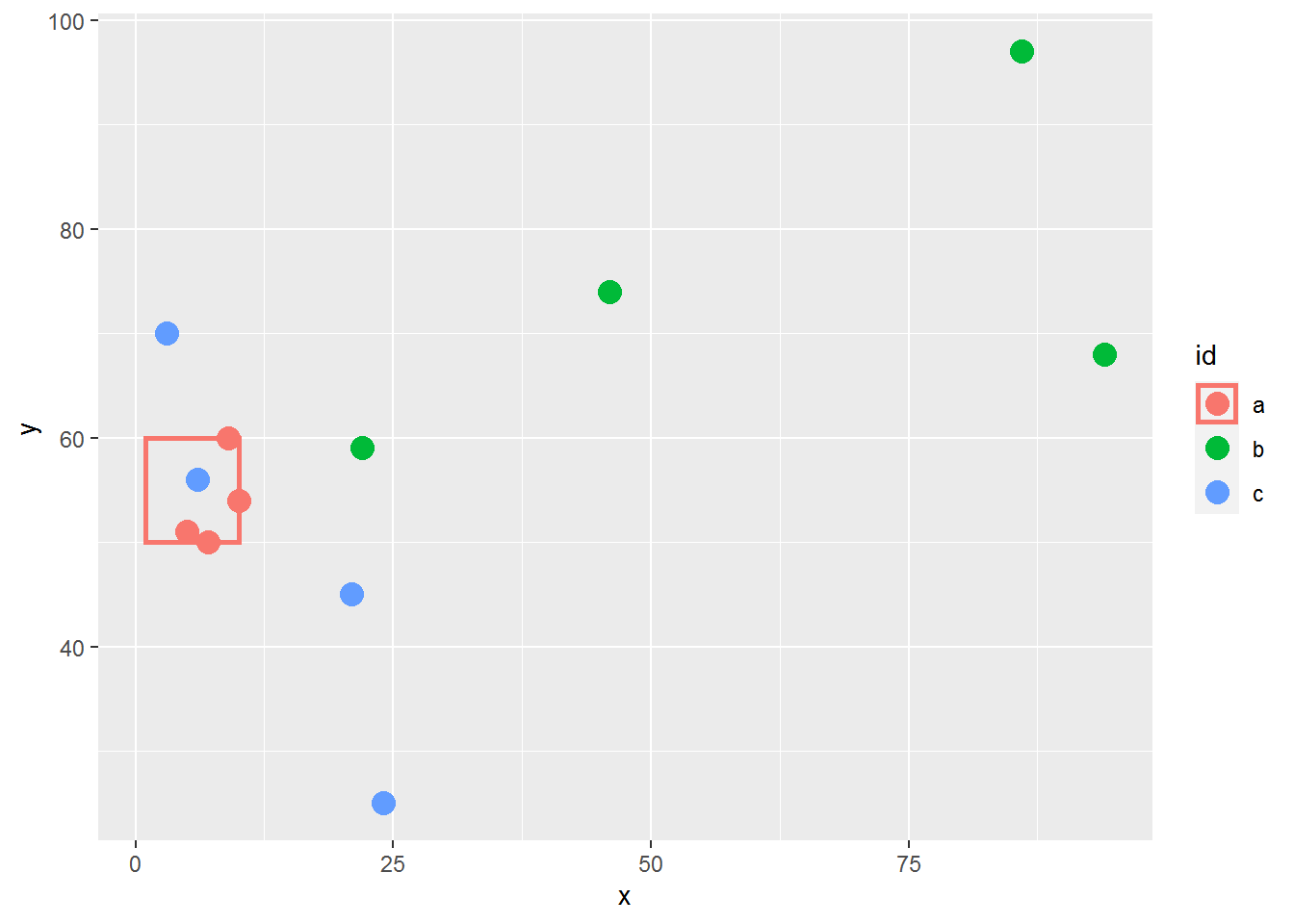
Combining legends from two layers
In the next example I’ll show how override.aes can be useful when creating a legend based on multiple layers and want distinct symbols in each legend key box.
There are situations where we want to add a legend to identify different elements of the plot, such as indicating the plotted line is a fitted line or that points are means. This can be done by mapping aesthetics to constants to make a manual legend and then manipulating the symbols shown in the legend via override.aes. I wrote about making manual legends in an earlier blog post.
The plot below shows observed values and a fitted line per group based on color.
ggplot(data = mtcars, aes(x = mpg, y = wt, color = factor(am) ) ) +
geom_point(size = 3) +
geom_smooth(method = "lm", se = FALSE)# `geom_smooth()` using formula 'y ~ x'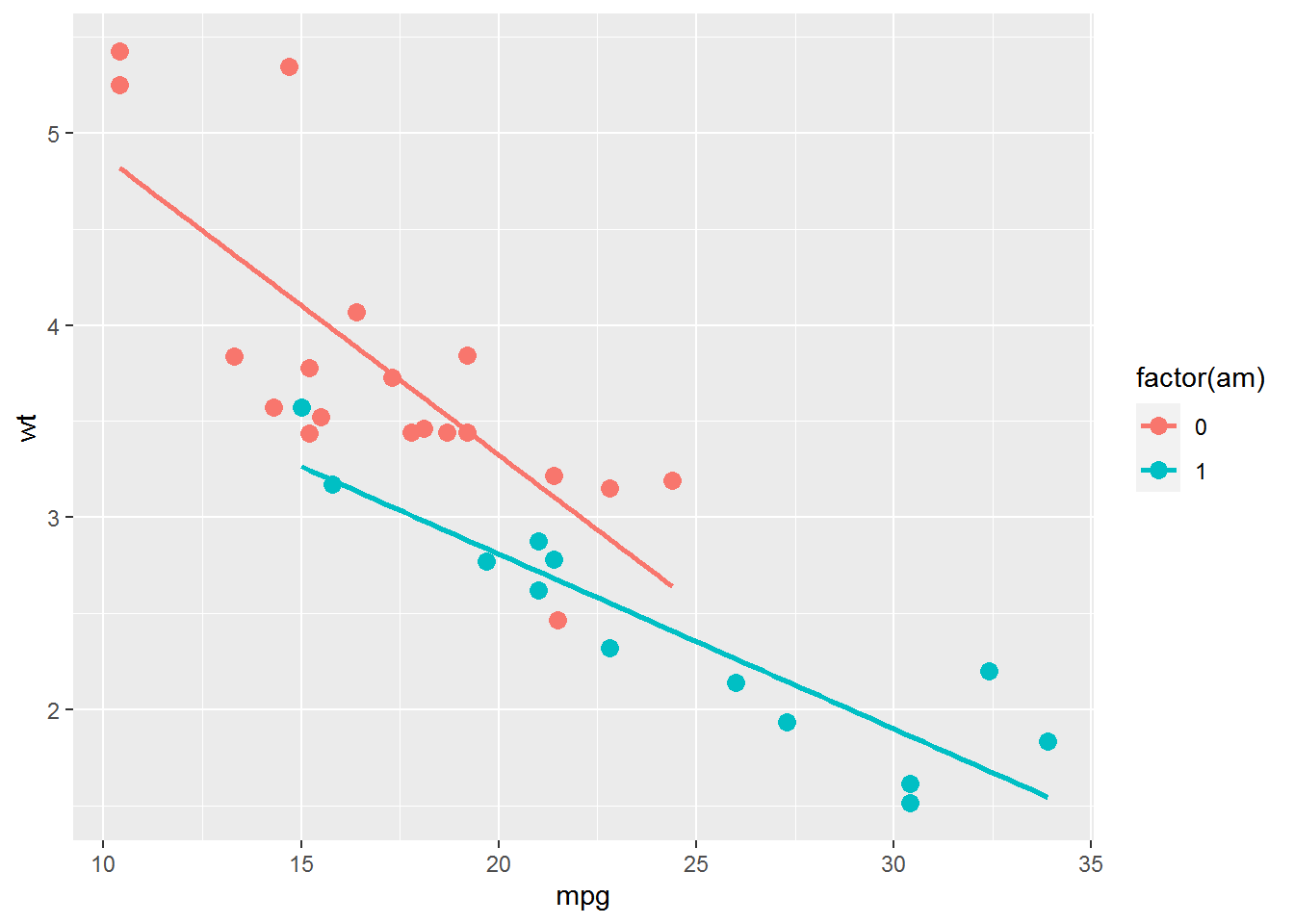
I’m going to leave the color legend alone but I want to add a second legend to indicate that the points are observed values and the lines are fitted lines. I’ll use the alpha aesthetic for this. Using an aesthetic that you haven’t used already and affects both layers is a trick that often comes in handy when adding an extra legend like I’m doing here.
I don’t actually want alpha to affect the plot appearance, so I also add scale_alpha_manual() to make sure both layers stay opaque by setting the values for both groups to 1. I also remove the legend name and set the order of the breaks so the Observed group is listed first in the new legend.
ggplot(data = mtcars, aes(x = mpg, y = wt, color = factor(am) ) ) +
geom_point(aes(alpha = "Observed"), size = 3) +
geom_smooth(method = "lm", se = FALSE, aes(alpha = "Fitted") ) +
scale_alpha_manual(name = NULL,
values = c(1, 1),
breaks = c("Observed", "Fitted") )
Now I have a new legend to work with. However, the legend has both the point and the line symbol in all legend key boxes. I need to override the current legend so the Observed legend key box contains only a point symbol and the Fitted legend key box has only a line symbol. This is where override.aes comes in.
Here’s what I’ll do: I’ll change the linetype to 0 for the first key box but leave it as 1 for the second. I’ll use shape 16 (a solid circle) as the shape for the first key box but remove the point all together in the second key box with NA. I’m also going to make sure all elements are black via color. (If you need to know codes for shapes and line types see here.)
I use linetype, shape, and color in the override.aes list within scale_alpha_manual().
ggplot(data = mtcars, aes(x = mpg, y = wt, color = factor(am) ) ) +
geom_point(aes(alpha = "Observed"), size = 3) +
geom_smooth(method = "lm", se = FALSE, aes(alpha = "Fitted") ) +
scale_alpha_manual(name = NULL,
values = c(1, 1),
breaks = c("Observed", "Fitted"),
guide = guide_legend(override.aes = list(linetype = c(0, 1),
shape = c(16, NA),
color = "black") ) )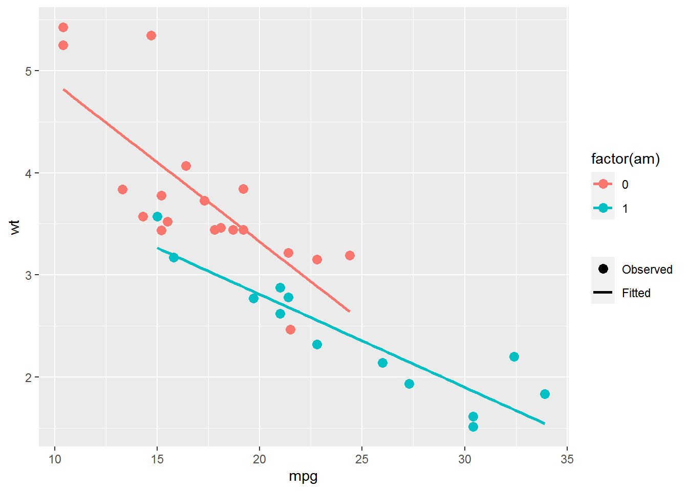
Controlling the appearance of multiple legends
The final example for override.aes may seem a little esoteric, but it has come up for me in the past. Say I want to make a scatterplot with the fill and shape aesthetics mapped to two different factors. I use fill instead of color so the points have an outline. Having an outline around the points can matter if, e.g., you have a white plot background and wanted the points to be black and white as in this question.
This is the dataset I’ll use in this plot example, where the two factors are named g1 and g2.
dat = structure(list(g1 = structure(c(1L, 2L, 1L, 2L, 1L, 2L, 1L, 2L,
1L, 2L, 1L, 2L, 1L, 2L, 1L, 2L), class = "factor", .Label = c("High",
"Low")), g2 = structure(c(1L, 1L, 2L, 2L, 1L, 1L, 2L, 2L, 1L,
1L, 2L, 2L, 1L, 1L, 2L, 2L), class = "factor", .Label = c("Control",
"Treatment")), x = c(0.42, 0.39, 0.56, 0.59, 0.17, 0.95, 0.85,
0.25, 0.31, 0.75, 0.58, 0.9, 0.6, 0.86, 0.61, 0.61), y = c(-1.4,
3.6, 1.1, -0.1, 0.5, 0, -1.8, 0.8, -1.1, -0.6, 0.2, 0.3, 1.1,
1.6, 0.9, -0.6)), class = "data.frame", row.names = c(NA, -16L
))
head(dat)# g1 g2 x y
# 1 High Control 0.42 -1.4
# 2 Low Control 0.39 3.6
# 3 High Treatment 0.56 1.1
# 4 Low Treatment 0.59 -0.1
# 5 High Control 0.17 0.5
# 6 Low Control 0.95 0.0I set the colors for the fill in scale_fill_manual() and choose fillable shapes in scale_shape_manual(). Fillable shapes are shapes 21 through 25.
ggplot(data = dat, aes(x = x, y = y, fill = g1, shape = g2) ) +
geom_point(size = 5) +
scale_fill_manual(values = c("#002F70", "#EDB4B5") ) +
scale_shape_manual(values = c(21, 24) )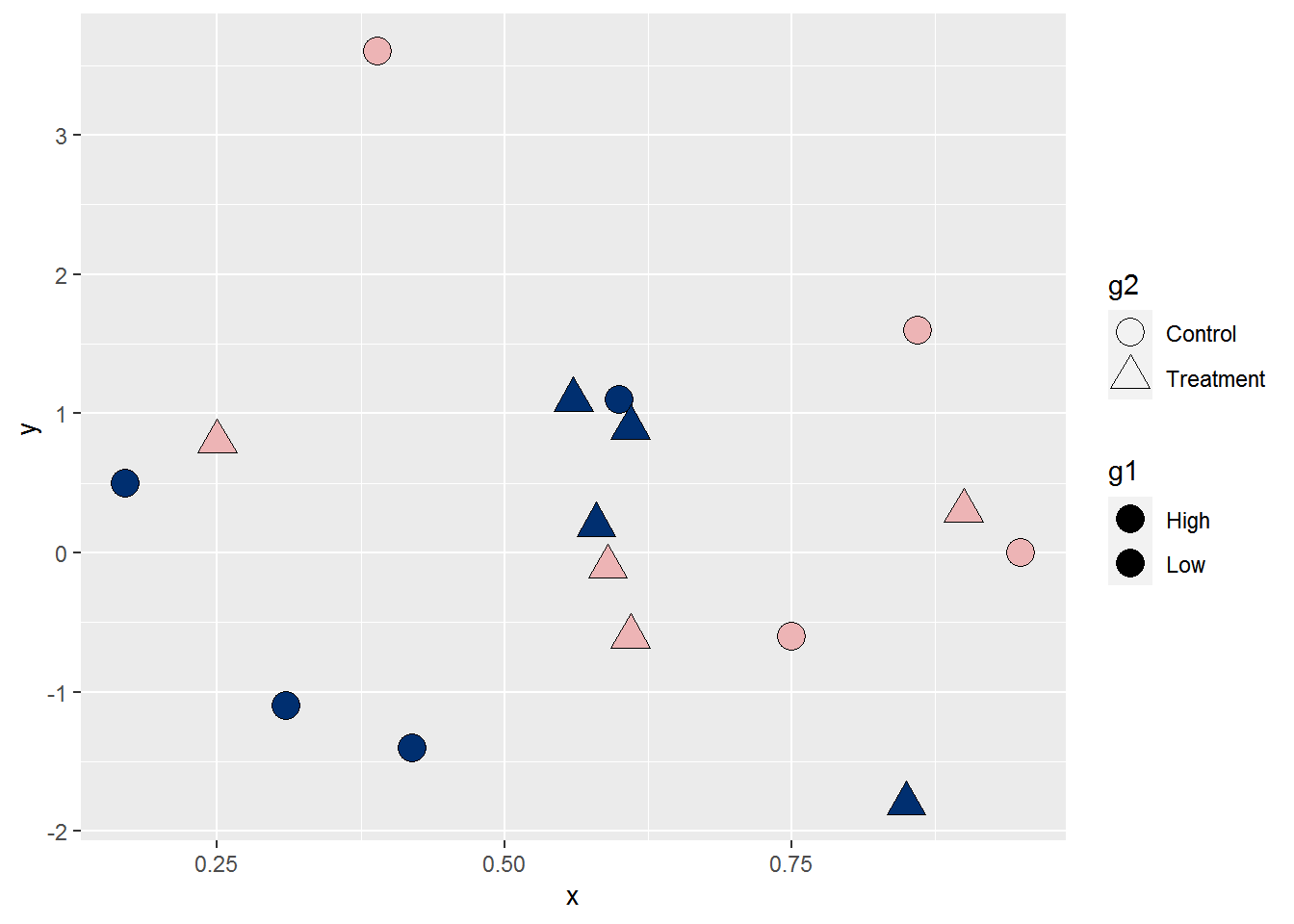
The plots itself shows the fill colors and shapes, but you can some issues in the legends. The fill colors don’t show up in the g1 legend at all. This is because the default shape in the legend isn’t a fillable shape. In addition, the g2 legend shows unfilled points and I think it would look better if the points were filled.
I can address both these issues via override.aes. I’ll change the point shape in the fill legend to shape 21 and the fill color in the shape legend to black within a guides() layer. This code gives you a chance to see how you can use use multiple scale name-guide pairs within the same guides() layer.
ggplot(data = dat, aes(x = x, y = y, fill = g1, shape = g2) ) +
geom_point(size = 5) +
scale_fill_manual(values = c("#002F70", "#EDB4B5") ) +
scale_shape_manual(values = c(21, 24) ) +
guides(fill = guide_legend(override.aes = list(shape = 21) ),
shape = guide_legend(override.aes = list(fill = "black") ) )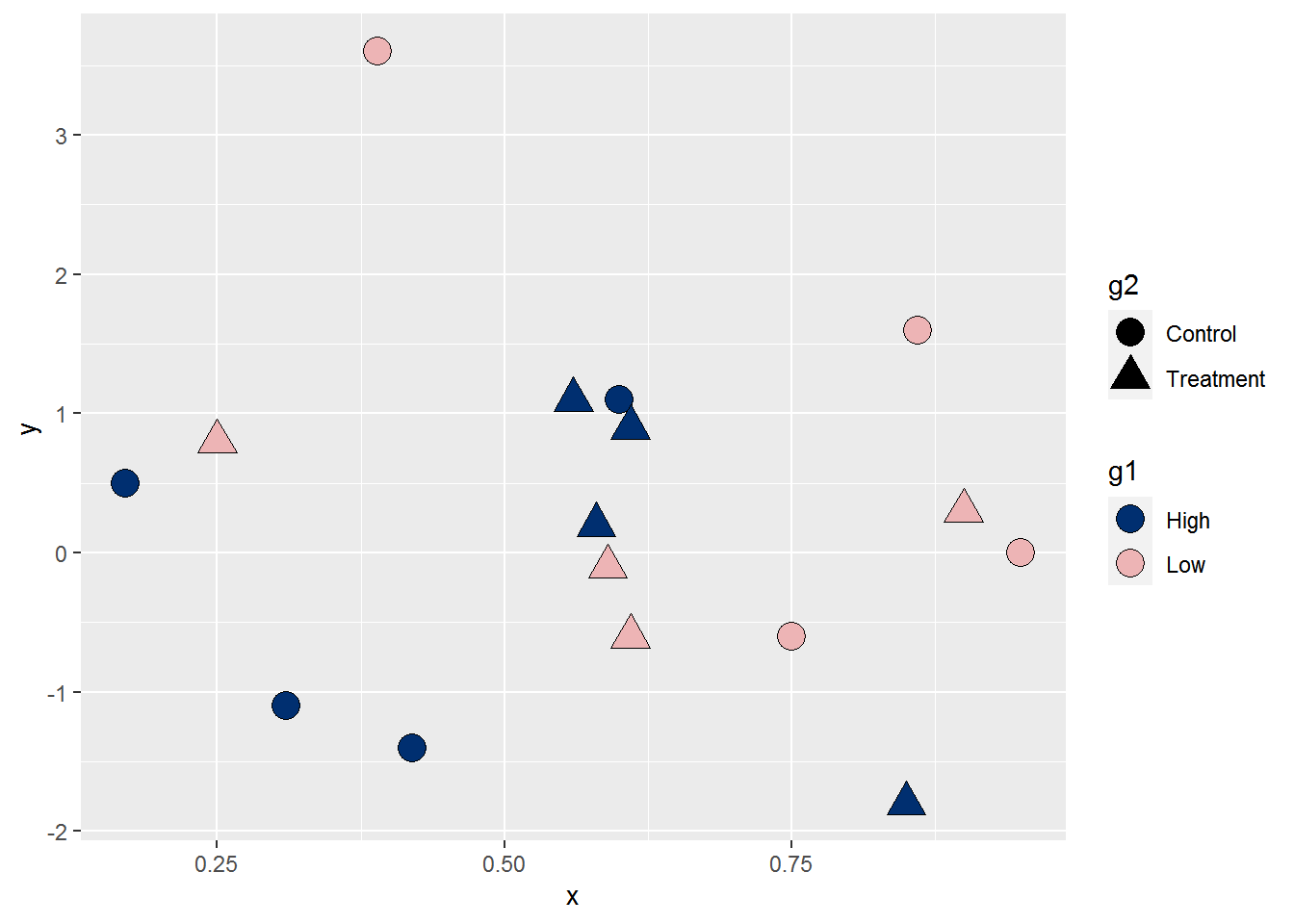
While I’m sure you can come up with additional scenarios, that should give you a taste for when overriding the aesthetics in the legend is useful. 😄
Just the code, please
Here’s the code without all the discussion. Copy and paste the code below or you can download an R script of uncommented code from here.
library(ggplot2) # v. 3.3.2
ggplot(data = diamonds, aes(x = carat, y = price, color = cut) ) +
geom_point(alpha = .25, size = 1)
ggplot(data = diamonds, aes(x = carat, y = price, color = cut) ) +
geom_point(alpha = .25, size = 1) +
guides(color = guide_legend(override.aes = list(size = 3) ) )
ggplot(data = diamonds, aes(x = carat, y = price, color = cut) ) +
geom_point(alpha = .25, size = 1) +
scale_color_viridis_d(option = "magma",
guide = guide_legend(override.aes = list(size = 3) ) )
ggplot(data = diamonds, aes(x = carat, y = price, color = cut) ) +
geom_point(alpha = .25, size = 1) +
scale_color_viridis_d(option = "magma",
guide = guide_legend(override.aes = list(size = 3,
alpha = 1) ) )
points = structure(list(x = c(5L, 10L, 7L, 9L, 86L, 46L, 22L, 94L, 21L,
6L, 24L, 3L), y = c(51L, 54L, 50L, 60L, 97L, 74L, 59L, 68L, 45L,
56L, 25L, 70L), id = c("a", "a", "a", "a", "b", "b", "b", "b",
"c", "c", "c", "c")), row.names = c(NA, -12L), class = "data.frame")
head(points)
box = data.frame(left = 1, right = 10, bottom = 50, top = 60, id = "a")
box
ggplot(data = points, aes(color = id) ) +
     geom_point(aes(x = x, y = y), size = 4) +
     geom_rect(data = box, aes(xmin = left,
                               xmax = right,
                               ymin = 50,
                               ymax = top),
               fill = NA, size = 1)
ggplot(data = points, aes(color = id) ) +
     geom_point(aes(x = x, y = y), size = 4) +
     geom_rect(data = box, aes(xmin = left,
                               xmax = right,
                               ymin = 50,
                               ymax = top),
               fill = NA, size = 1) +
     guides(color = guide_legend(override.aes = list(linetype = c(1, 0, 0) ) ) )
ggplot(data = mtcars, aes(x = mpg, y = wt, color = factor(am) ) ) +
     geom_point(size = 3) +
     geom_smooth(method = "lm", se = FALSE)
ggplot(data = mtcars, aes(x = mpg, y = wt, color = factor(am) ) ) +
     geom_point(aes(alpha = "Observed"), size = 3) +
     geom_smooth(method = "lm", se = FALSE, aes(alpha = "Fitted") ) +
     scale_alpha_manual(name = NULL,
                        values = c(1, 1),
                        breaks = c("Observed", "Fitted") )
ggplot(data = mtcars, aes(x = mpg, y = wt, color = factor(am) ) ) +
     geom_point(aes(alpha = "Observed"), size = 3) +
     geom_smooth(method = "lm", se = FALSE, aes(alpha = "Fitted") ) +
     scale_alpha_manual(name = NULL,
                        values = c(1, 1),
                        breaks = c("Observed", "Fitted"),
                        guide = guide_legend(override.aes = list(linetype = c(0, 1),
                                                                  shape = c(16, NA),
                                                                  color = "black") ) )
dat = structure(list(g1 = structure(c(1L, 2L, 1L, 2L, 1L, 2L, 1L, 2L,
1L, 2L, 1L, 2L, 1L, 2L, 1L, 2L), class = "factor", .Label = c("High",
"Low")), g2 = structure(c(1L, 1L, 2L, 2L, 1L, 1L, 2L, 2L, 1L,
1L, 2L, 2L, 1L, 1L, 2L, 2L), class = "factor", .Label = c("Control",
"Treatment")), x = c(0.42, 0.39, 0.56, 0.59, 0.17, 0.95, 0.85,
0.25, 0.31, 0.75, 0.58, 0.9, 0.6, 0.86, 0.61, 0.61), y = c(-1.4,
3.6, 1.1, -0.1, 0.5, 0, -1.8, 0.8, -1.1, -0.6, 0.2, 0.3, 1.1,
1.6, 0.9, -0.6)), class = "data.frame", row.names = c(NA, -16L
))

head(dat)
ggplot(data = dat, aes(x = x, y = y, fill = g1, shape = g2) ) +
     geom_point(size = 5) +
     scale_fill_manual(values = c("#002F70", "#EDB4B5") ) +
     scale_shape_manual(values = c(21, 24) )
ggplot(data = dat, aes(x = x, y = y, fill = g1, shape = g2) ) +
     geom_point(size = 5) +
     scale_fill_manual(values = c("#002F70", "#EDB4B5") ) +
     scale_shape_manual(values = c(21, 24) ) +
     guides(fill = guide_legend(override.aes = list(shape = 21) ),
            shape = guide_legend(override.aes = list(fill = "black") ) )